空売り比率と日経平均株価
Updated time:2020-01-15 09:22:20
- Source:日本取引所グループ、日本経済新聞社
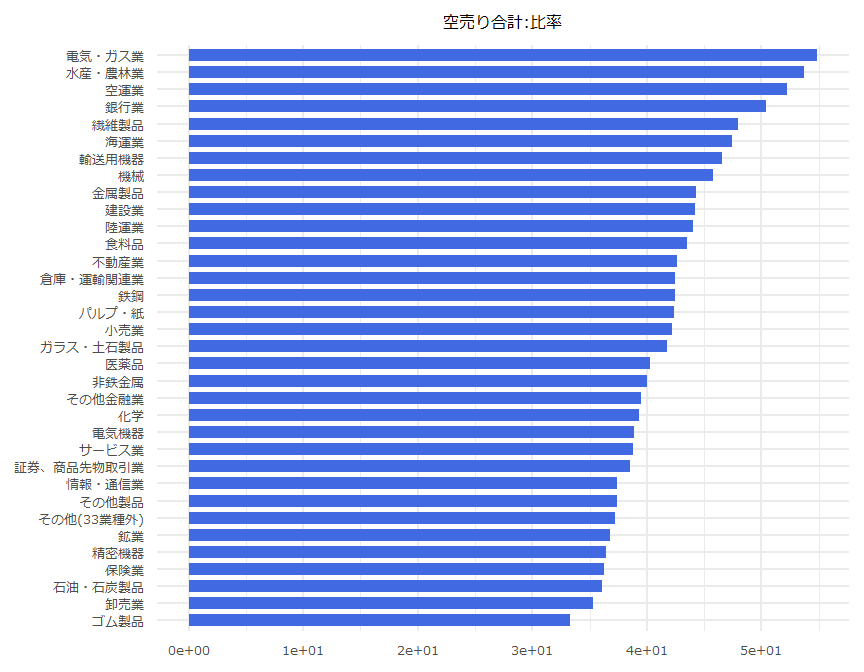
| N | 業種名 | 空売り合計:比率 |
|---|---|---|
| 1 | 水産・農林業 | 53.7 |
| 2 | 鉱業 | 36.8 |
| 3 | 建設業 | 44.2 |
| 4 | 食料品 | 43.5 |
| 5 | 繊維製品 | 48 |
| 6 | パルプ・紙 | 42.4 |
| 7 | 化学 | 39.3 |
| 8 | 医薬品 | 40.3 |
| 9 | 石油・石炭製品 | 36.1 |
| 10 | ゴム製品 | 33.3 |
| 11 | ガラス・土石製品 | 41.8 |
| 12 | 鉄鋼 | 42.5 |
| 13 | 非鉄金属 | 40 |
| 14 | 金属製品 | 44.3 |
| 15 | 機械 | 45.8 |
| 16 | 電気機器 | 38.9 |
| 17 | 輸送用機器 | 46.6 |
| 18 | 精密機器 | 36.4 |
| 19 | その他製品 | 37.4 |
| 20 | 電気・ガス業 | 54.9 |
| 21 | 陸運業 | 44 |
| 22 | 海運業 | 47.4 |
| 23 | 空運業 | 52.2 |
| 24 | 倉庫・運輸関連業 | 42.5 |
| 25 | 情報・通信業 | 37.4 |
| 26 | 卸売業 | 35.3 |
| 27 | 小売業 | 42.2 |
| 28 | 銀行業 | 50.4 |
| 29 | 証券、商品先物取引業 | 38.5 |
| 30 | 保険業 | 36.3 |
| 31 | その他金融業 | 39.5 |
| 32 | 不動産業 | 42.6 |
| 33 | サービス業 | 38.8 |
| 34 | その他(33業種外) | 37.2 |
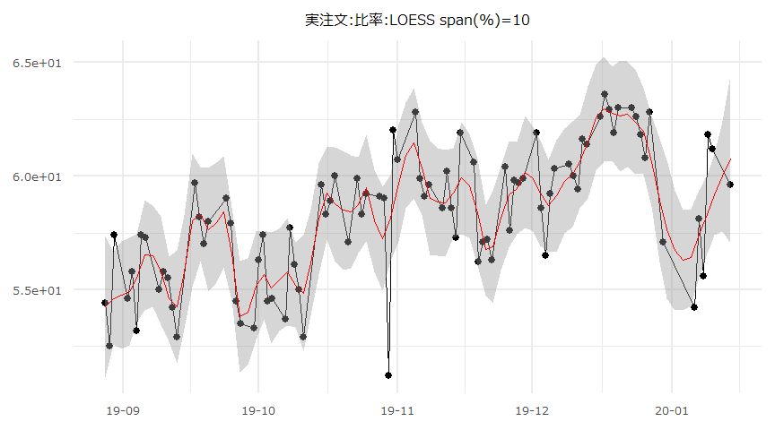
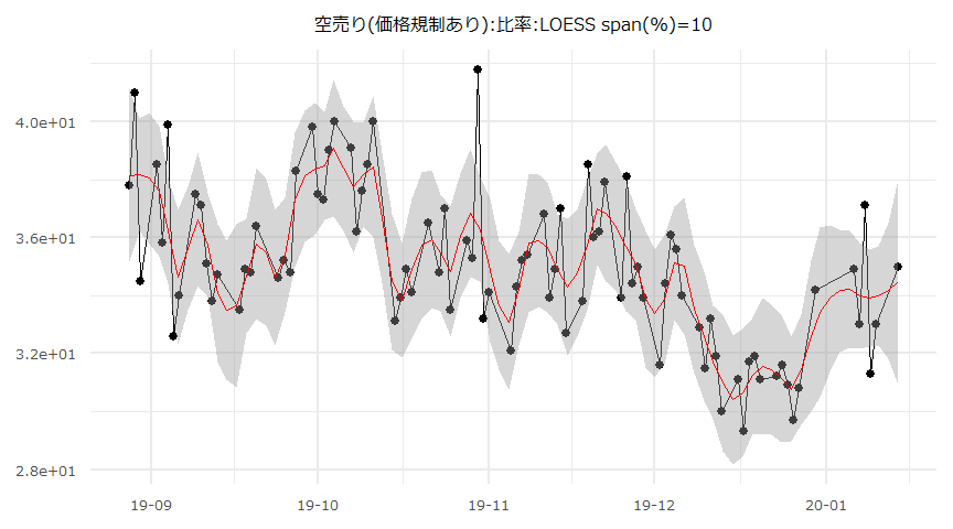
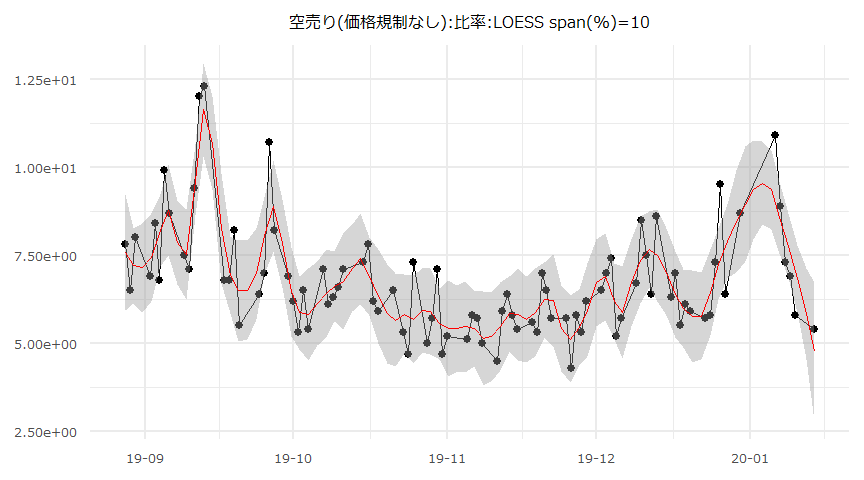
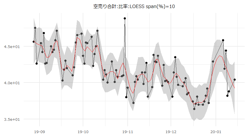
空売り比率の時系列推移
- 2019-08-28 ~ 2020-01-14
| Date | 01-14 | 01-10 | 01-09 | 01-08 | 01-07 | 01-06 | 12-30 | 12-27 |
|---|---|---|---|---|---|---|---|---|
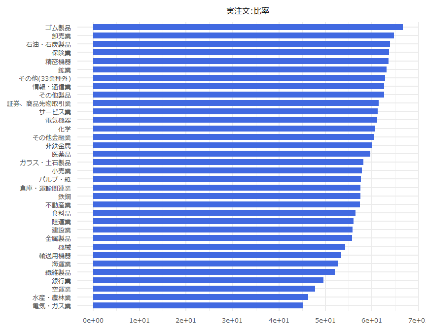
| 実注文:比率 | 59.6 | 61.2 | 61.8 | 55.6 | 58.1 | 54.2 | 57.1 | 62.8 |
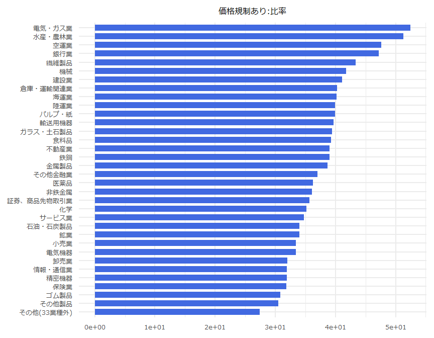
| 空売り(価格規制あり):比率 | 35 | 33 | 31.3 | 37.1 | 33 | 34.9 | 34.2 | 30.8 |
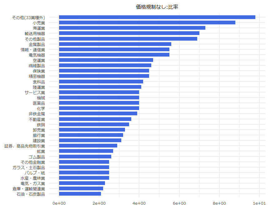
| 空売り(価格規制なし):比率 | 5.4 | 5.8 | 6.9 | 7.3 | 8.9 | 10.9 | 8.7 | 6.4 |
| 空売り合計:比率 | 40.4 | 38.8 | 38.2 | 44.4 | 41.9 | 45.8 | 42.9 | 37.2 |
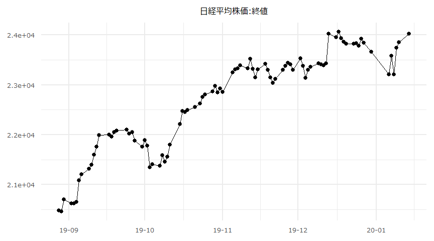
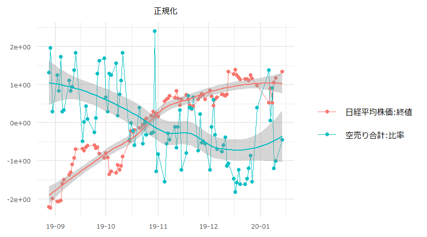
日経平均株価と空売り比率
時系列推移
- 対象期間:2019-08-28 ~ 2020-01-14
単位根検定/共和分検定
- CADFtest {CADFtest}
- ca.po {urca}
- 各系列の“_change“は前営業日との差。
- 対象期間: 2019-08-28 ~ 2020-01-14,90days
### 単位根検定 ###

$NIKKEI225.close

    ADF test

data:  x
ADF(0) = -2.5292, p-value = 0.3137
alternative hypothesis: true delta is less than 0
sample estimates:
     delta
-0.1289646


$ShortSalerRatio

    ADF test

data:  x
ADF(0) = -6.7065, p-value = 0.0000007748
alternative hypothesis: true delta is less than 0
sample estimates:
     delta
-0.6963772


$NIKKEI225.close_change

    ADF test

data:  x
ADF(0) = -10.04, p-value = 0.00000000000369
alternative hypothesis: true delta is less than 0
sample estimates:
    delta
-1.090583


$ShortSalerRatio_change

    ADF test

data:  x
ADF(2) = -8.2208, p-value = 0.000000002009
alternative hypothesis: true delta is less than 0
sample estimates:
    delta
-2.103106
### 共和分検定 ###
########################################
# Phillips and Ouliaris Unit Root Test #
########################################
Test of type Pu
detrending of series none
Call:
lm(formula = z[, 1] ~ z[, -1] - 1)
Residuals:
Min 1Q Median 3Q Max
-5175.8 -1810.0 445.8 1925.6 4420.3
Coefficients:
Estimate Std. Error t value Pr(>|t|)
z[, -1] 539.720 6.075 88.84 <0.0000000000000002 ***
---
Signif. codes: 0 '***' 0.001 '**' 0.01 '*' 0.05 '.' 0.1 ' ' 1
Residual standard error: 2411 on 89 degrees of freedom
Multiple R-squared: 0.9889, Adjusted R-squared: 0.9887
F-statistic: 7893 on 1 and 89 DF, p-value: < 0.00000000000000022
Value of test-statistic is: 0.3606
Critical values of Pu are:
10pct 5pct 1pct
critical values 20.3933 25.9711 38.3413最小二乗法
- lm {stats}
- dwtest {lmtest}
- ks.test {stats}
- confint {stats}
- Box.test {stats}
- Ljung-Box 検定のラグは15としている。
- 対象期間: 2019-08-28 ~ 2020-01-14,90days
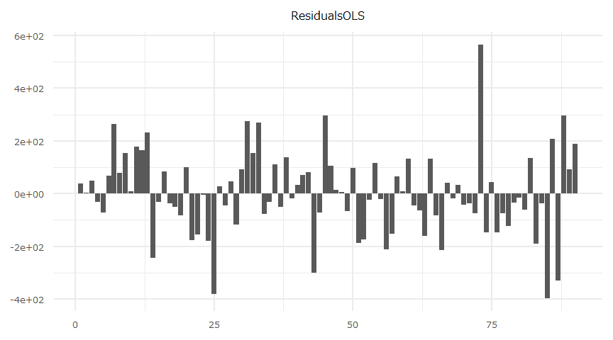
- 切片項\(\neq0\)
Call:
lm(formula = NIKKEI225.close_change ~ ShortSalerRatio_change,
    data = datadf)

Residuals:
    Min      1Q  Median      3Q     Max
-397.06  -76.04  -17.09   92.27  566.30

Coefficients:
                       Estimate Std. Error t value    Pr(>|t|)
(Intercept)              38.408     16.609   2.313      0.0231 *
ShortSalerRatio_change  -32.107      6.074  -5.286 0.000000901 ***
---
Signif. codes:  0 '***' 0.001 '**' 0.01 '*' 0.05 '.' 0.1 ' ' 1

Residual standard error: 157.5 on 88 degrees of freedom
Multiple R-squared:  0.241, Adjusted R-squared:  0.2323
F-statistic: 27.94 on 1 and 88 DF,  p-value: 0.0000009009
    Durbin-Watson test

data:  OLS_Model
DW = 2.0825, p-value = 0.6685
alternative hypothesis: true autocorrelation is greater than 0
    One-sample Kolmogorov-Smirnov test

data:  ResidualsOLS
D = 0.088908, p-value = 0.4496
alternative hypothesis: two-sided
2.5 % 97.5 %
(Intercept) 5.401937 71.41393
ShortSalerRatio_change -44.179109 -20.03574
Box-Ljung test
data: ResidualsOLS
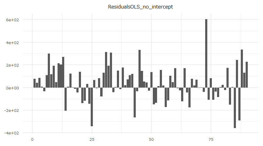
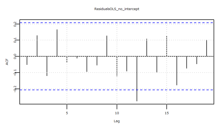
X-squared = 23.312, df = 15, p-value = 0.07773- 切片項\(=0\)
Call:
lm(formula = NIKKEI225.close_change ~ ShortSalerRatio_change -
    1, data = datadf)

Residuals:
    Min      1Q  Median      3Q     Max
-358.07  -37.91   21.26  130.87  604.75

Coefficients:
                       Estimate Std. Error t value   Pr(>|t|)
ShortSalerRatio_change   -32.31       6.22  -5.194 0.00000129 ***
---
Signif. codes:  0 '***' 0.001 '**' 0.01 '*' 0.05 '.' 0.1 ' ' 1

Residual standard error: 161.3 on 89 degrees of freedom
Multiple R-squared:  0.2326,    Adjusted R-squared:  0.224
F-statistic: 26.97 on 1 and 89 DF,  p-value: 0.000001294
    Durbin-Watson test

data:  OLS_Model_no_intercept
DW = 1.964, p-value = 0.4919
alternative hypothesis: true autocorrelation is greater than 0
    One-sample Kolmogorov-Smirnov test

data:  ResidualsOLS_no_intercept
D = 0.18037, p-value = 0.004928
alternative hypothesis: two-sided
2.5 % 97.5 %
ShortSalerRatio_change -44.66707 -19.94738
    Box-Ljung test

data:  ResidualsOLS_no_intercept
X-squared = 23.293, df = 15, p-value = 0.07812
一般化最小二乗法
- gls {nlme}
- corARMA {nlme}
- ks.test {stats}
- confint {stats}
- Box.test {stats}
- 残差の系列相関の有無に拘わらず一般化最小二乗法による回帰係数を求めています。
- 最小二乗法の残差に系列相関が見られない場合、ここではAR(p=0,q=0)の結果(AIC最小)が表示されます。
- http://user.keio.ac.jp/~nagakura/zemi/GLS.pdf
- http://tokyox.matrix.jp/wiki/index.php?%E4%B8%80%E8%88%AC%E5%8C%96%E6%9C%80%E5%B0%8F%E4%BA%8C%E4%B9%97%E6%B3%95
- Ljung-Box 検定のラグは15としている。
- 切片項\(\neq0\)
Generalized least squares fit by REML
  Model: NIKKEI225.close_change ~ ShortSalerRatio_change
  Data: datadf
       AIC      BIC    logLik
  1157.255 1164.687 -575.6276

Coefficients:
                           Value Std.Error   t-value p-value
(Intercept)             38.40793 16.608547  2.312540  0.0231
ShortSalerRatio_change -32.10742  6.074446 -5.285655  0.0000

 Correlation:
                       (Intr)
ShortSalerRatio_change 0.014

Standardized residuals:
       Min         Q1        Med         Q3        Max
-2.5202478 -0.4826562 -0.1085063  0.5856795  3.5945152

Residual standard error: 157.5466
Degrees of freedom: 90 total; 88 residual
    One-sample Kolmogorov-Smirnov test

data:  ResidualsGLS
D = 0.088908, p-value = 0.4496
alternative hypothesis: two-sided
2.5 % 97.5 %
(Intercept) 5.85578 70.96009
ShortSalerRatio_change -44.01312 -20.20173
    Box-Ljung test

data:  ResidualsGLS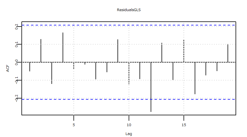
X-squared = 23.312, df = 15, p-value = 0.07773- 切片項\(=0\)
Generalized least squares fit by REML
  Model: NIKKEI225.close_change ~ ShortSalerRatio_change - 1
  Data: datadf
       AIC      BIC    logLik
  1167.958 1172.935 -581.9789

Coefficients:
                           Value Std.Error   t-value p-value
ShortSalerRatio_change -32.30722  6.220422 -5.193735       0

Standardized residuals:
       Min         Q1        Med         Q3        Max
-2.2192217 -0.2349728  0.1317839  0.8111274  3.7480970

Residual standard error: 161.3489
Degrees of freedom: 90 total; 89 residual
    One-sample Kolmogorov-Smirnov test

data:  ResidualsGLS_no_intercept
D = 0.18037, p-value = 0.004928
alternative hypothesis: two-sided
2.5 % 97.5 %
ShortSalerRatio_change -44.49903 -20.11542
    Box-Ljung test

data:  ResidualsGLS_no_intercept
X-squared = 23.293, df = 15, p-value = 0.07812
残差
- 時系列推移
- 自己相関
- 時系列推移


- 自己相関


業種別空売り集計