Rでデータサイズ:国土数値情報(国土交通省)の行政区域シェープファイルを利用して都道府県境界のシェープファイルとGeoJSONおよび都道府県境界コロプレスマップを作成するためのRスクリプト

Rでデータサイエンス

geojsonファイルへのリンク

下記リンクは本ページのRスクリプトにより作成した、日本の都道府県境界GeoJSONファイルです。
1. 許容誤差は1000mに単純化しています。
2. 日本全体版:https://am-consulting.co.jp/simple_japanmap_01.geojson
3. コロプレスマップのための部分的非表示化と沖縄県の拡大および移動版:https://am-consulting.co.jp/simple_japanmap_02.geojson

国土数値情報データの読み込み

事前に「国土数値情報ダウンロードサイト」(https://nlftp.mlit.go.jp/ksj/gml/datalist/KsjTmplt-N03-2024.html)から「N03-20240101_GML.zip」(全国データ)をダウンロード、展開してあるとします。
本ページでは下記のフォルダ「dir_shapefile」を展開先としています。
https://stackoverflow.com/questions/75927165/error-in-wk-handle-wk-wkbwkb-s2-geography-writeroriented-oriented-loop-0

library(dplyr)
library(sf)
packageVersion("sf")

[1] '1.0.16'

dir_shapefile <- "D:/N03-20240101_GML"
dir_shapefile %>%
    setwd()
dir(pattern = "N03-20240101")

 [1] "KS-META-N03-20240101.xml"            "KS-META-N03-20240101_prefecture.xml"
 [3] "N03-20240101.cpg"                    "N03-20240101.dbf"                   
 [5] "N03-20240101.geojson"                "N03-20240101.prj"                   
 [7] "N03-20240101.shp"                    "N03-20240101.shx"                   
 [9] "N03-20240101.xml"                    "N03-20240101_prefecture.cpg"        
[11] "N03-20240101_prefecture.dbf"         "N03-20240101_prefecture.geojson"    
[13] "N03-20240101_prefecture.prj"         "N03-20240101_prefecture.shp"        
[15] "N03-20240101_prefecture.shx"         "N03-20240101_prefecture.xml"

dir_shapefile %>%
    setwd()
japanshp <- read_sf("N03-20240101.shp", options = "ENCODING=UTF-8")
japanshp$Pref_code <- japanshp$N03_007 %>%
    substr(start = 1, stop = 2)

class(japanshp)

[1] "sf"         "tbl_df"     "tbl"        "data.frame"

japanshp %>%
    head()

Simple feature collection with 6 features and 7 fields
Geometry type: POLYGON
Dimension:     XY
Bounding box:  xmin: 140.9905 ymin: 42.78071 xmax: 141.4735 ymax: 43.18951
Geodetic CRS:  JGD2011
# A tibble: 6 × 8
  N03_001 N03_002    N03_003 N03_004 N03_005 N03_007                    geometry
  <chr>   <chr>      <chr>   <chr>   <chr>   <chr>                 <POLYGON [°]>
1 北海道  石狩振興局 <NA>    札幌市  中央区  01101   ((141.2569 42.99782, 141.2…
2 北海道  石狩振興局 <NA>    札幌市  北区    01102   ((141.3333 43.07505, 141.3…
3 北海道  石狩振興局 <NA>    札幌市  東区    01103   ((141.3734 43.0684, 141.37…
4 北海道  石狩振興局 <NA>    札幌市  白石区  01104   ((141.382 43.04832, 141.38…
5 北海道  石狩振興局 <NA>    札幌市  豊平区  01105   ((141.3637 42.94154, 141.3…
6 北海道  石狩振興局 <NA>    札幌市  南区    01106   ((141.2354 42.82273, 141.2…
# ℹ 1 more variable: Pref_code <chr>

japanshp %>%
    tail()

Simple feature collection with 6 features and 7 fields
Geometry type: POLYGON
Dimension:     XY
Bounding box:  xmin: 122.933 ymin: 24.43985 xmax: 122.9988 ymax: 24.45177
Geodetic CRS:  JGD2011
# A tibble: 6 × 8
  N03_001 N03_002 N03_003  N03_004  N03_005 N03_007                     geometry
  <chr>   <chr>   <chr>    <chr>    <chr>   <chr>                  <POLYGON [°]>
1 沖縄県  <NA>    八重山郡 与那国町 <NA>    47382   ((122.9347 24.44785, 122.93…
2 沖縄県  <NA>    八重山郡 与那国町 <NA>    47382   ((122.933 24.4517, 122.933 …
3 沖縄県  <NA>    八重山郡 与那国町 <NA>    47382   ((122.934 24.4482, 122.934 …
4 沖縄県  <NA>    八重山郡 与那国町 <NA>    47382   ((122.9421 24.44395, 122.94…
5 沖縄県  <NA>    八重山郡 与那国町 <NA>    47382   ((122.9988 24.43985, 122.99…
6 沖縄県  <NA>    八重山郡 与那国町 <NA>    47382   ((122.9331 24.45176, 122.93…
# ℹ 1 more variable: Pref_code <chr>

都道府県毎に1行に集約

参考資料
1. https://r-spatial.github.io/sf/reference/aggregate.sf.html
2. https://notchained.hatenablog.com/entry/2017/09/13/102358

# 『aggregate an sf object, possibly union-ing geometries』
raw_japanmap <- 
  aggregate(x = japanshp[,"Pref_code","geometry"],
            by = list(japanshp$Pref_code),
            FUN = function(x)length(x = x), # 1都道府県当たりの結合した行数
            do_union = TRUE, # logical; should grouped geometries be unioned using st_union?
            simplify = TRUE)
setwd(dir_shapefile)
st_write(obj = raw_japanmap,dsn = 'raw_japanmap.shp',layer_options = "ENCODING=UTF-8",delete_dsn = T)
beepr::beep(sound = 1)

setwd(dir_shapefile)
raw_japanmap <- read_sf("raw_japanmap.shp", options = "ENCODING=UTF-8")

シェープデータの簡素化

参考資料
1. https://keita43a.hatenablog.com/entry/2020/04/27/023918
2. https://www.r-bloggers.com/2021/03/simplifying-geospatial-features-in-r-with-sf-and-rmapshaper/

# 許容誤差を1000mとする。
simple_japanmap <- st_simplify(x = raw_japanmap, dTolerance = 1000, preserveTopology = TRUE)
setwd(dir_shapefile)
st_write(obj = simple_japanmap, dsn = "simple_japanmap.shp", layer_options = "ENCODING=UTF-8", delete_dsn = T)
beepr::beep(sound = 1)

setwd(dir_shapefile)
simple_japanmap <- read_sf("simple_japanmap.shp", options = "ENCODING=UTF-8")
colnames(simple_japanmap)[1:2] <- c("prefID", "row_count")
simple_japanmap

Simple feature collection with 47 features and 2 fields
Geometry type: MULTIPOLYGON
Dimension:     XY
Bounding box:  xmin: 122.9432 ymin: 24.04731 xmax: 148.8908 ymax: 45.55262
Geodetic CRS:  JGD2011
# A tibble: 47 × 3
   prefID row_count                                                     geometry
   <chr>      <int>                                           <MULTIPOLYGON [°]>
 1 01          9560 (((139.3382 41.50194, 139.3354 41.51359, 139.3515 41.52363,…
 2 02          2305 (((139.8807 40.58376, 139.8591 40.60252, 139.8706 40.62111,…
 3 03          8224 (((141.1046 38.82424, 141.1184 38.83601, 141.1457 38.86455,…
 4 04          8339 (((141.5232 38.39524, 141.5338 38.40306, 141.5379 38.38628,…
 5 05          2464 (((139.699 40.00305, 139.7098 39.99953, 139.7143 39.99087, …
 6 06           721 (((139.5406 39.18333, 139.5388 39.19245, 139.5454 39.21067,…
 7 07           229 (((140.4974 36.81926, 140.4727 36.79528, 140.4511 36.80644,…
 8 08           220 (((140.6361 36.41667, 140.625 36.43121, 140.61 36.4313, 140…
 9 09            28 (((139.7505 36.21238, 139.6911 36.20594, 139.6806 36.20053,…
10 10            37 (((138.7145 35.98672, 138.686 36.00078, 138.6379 36.02694, …
# ℹ 37 more rows

日本全体のマップ出力

library(ggplot2)
ggplot() + geom_sf(data = simple_japanmap)

geojsonファイルとして出力

library(geojsonsf)
simple_japanmap_01.geojson <- st_as_sf(x = simple_japanmap)
class(simple_japanmap_01.geojson)

[1] "sf"         "tbl_df"     "tbl"        "data.frame"

setwd(dir_shapefile)
st_write(simple_japanmap_01.geojson, "simple_japanmap_01.geojson", delete_dsn = T)

Deleting source `simple_japanmap_01.geojson' using driver `GeoJSON'
Writing layer `simple_japanmap_01' to data source 
  `simple_japanmap_01.geojson' using driver `GeoJSON'
Writing 47 features with 2 fields and geometry type Multi Polygon.

setwd(dir_shapefile)
simple_japanmap_01.geojson <- read_sf("simple_japanmap_01.geojson")
ggplot() + geom_sf(data = simple_japanmap_01.geojson)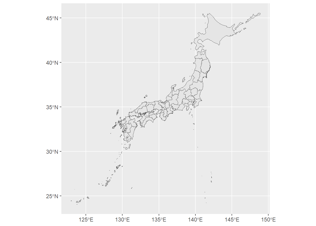

コロプレスマップのための部分的非表示化と沖縄県の移動

参考資料
1. https://rstudio-pubs-static.s3.amazonaws.com/775867_4cfbe983012a46cab16e53205452d3c8.html

東京都島嶼部

# (simple_japanmap$geometry[13] <-
# st_crop(x = simple_japanmap$geometry[13],y = c(xmin = 125, xmax = 150, ymin = 35, ymax = 90)))
# 20231031 修正
(simple_japanmap$geometry[13] <- st_crop(x = simple_japanmap$geometry[13], y = c(xmin = 125, xmax = 150, ymin = 30, ymax = 90)))
ggplot() + geom_sf(data = simple_japanmap)

Geometry set for 1 feature 
Geometry type: MULTIPOLYGON
Dimension:     XY
Bounding box:  xmin: 138.9458 ymin: 32.44661 xmax: 139.9153 ymax: 35.89712
Geodetic CRS:  JGD2011

鹿児島県島嶼部

# (simple_japanmap$geometry[46] <-
# st_crop(x = simple_japanmap$geometry[46],y = c(xmin = 125, xmax = 150, ymin = 30.9, ymax = 90)))
# 20231031 修正
(simple_japanmap$geometry[46] <- st_crop(x = simple_japanmap$geometry[46], y = c(xmin = 125, xmax = 150, ymin = 28.5, ymax = 90)))
ggplot() + geom_sf(data = simple_japanmap)

Geometry set for 1 feature 
Geometry type: MULTIPOLYGON
Dimension:     XY
Bounding box:  xmin: 129.1862 ymin: 29.13424 xmax: 131.2047 ymax: 32.30436
Geodetic CRS:  JGD2011

沖縄本島およびその近辺以外

(simple_japanmap$geometry[47] <- st_crop(x = simple_japanmap$geometry[47], y = c(xmin = 127.5, xmax = 150, ymin = 26, ymax = 26.89)))
ggplot() + geom_sf(data = simple_japanmap)

Geometry set for 1 feature 
Geometry type: MULTIPOLYGON
Dimension:     XY
Bounding box:  xmin: 127.6317 ymin: 26.08155 xmax: 128.3273 ymax: 26.92545
Geodetic CRS:  JGD2011

沖縄本島の拡大と移動

拡大と移動

okinawa01 <- simple_japanmap$geometry[47]
center_of_okinawa <- sf::st_centroid(okinawa01)
zoom_rate <- 3  # 拡大率
position_shift <- c(5, 15)  # c(経度,緯度) 東に5度、北に15度移動。
simple_japanmap$geometry[47] <- (okinawa01 - center_of_okinawa) * zoom_rate + center_of_okinawa + position_shift
ggplot() + geom_sf(data = simple_japanmap)

geojsonファイルとして出力

simple_japanmap_02.geojson <- st_as_sf(x = simple_japanmap)
class(simple_japanmap_02.geojson)

[1] "sf"         "tbl_df"     "tbl"        "data.frame"

setwd(dir_shapefile)
st_write(simple_japanmap_02.geojson, "simple_japanmap_02.geojson", delete_dsn = T)

Deleting source `simple_japanmap_02.geojson' using driver `GeoJSON'
Writing layer `simple_japanmap_02' to data source 
  `simple_japanmap_02.geojson' using driver `GeoJSON'
Writing 47 features with 2 fields and geometry type Multi Polygon.

setwd(dir_shapefile)
simple_japanmap_02.geojson <- read_sf("simple_japanmap_02.geojson")
ggplot() + geom_sf(data = simple_japanmap_02.geojson)

枠線の表示

func_add_segment_to_shp_map <- function(x = c(129, 132.5, 136), xend = c(132.5, 136, 136), y = c(39, 39, 42), yend = c(39, 42, 44), size = ggplot2::.pt/15) {
    ggplot2::annotate("segment", x = x, xend = xend, y = y, yend = yend, linewidth = .pt/15)
}
ggplot() + geom_sf(data = simple_japanmap) + func_add_segment_to_shp_map() + theme(axis.title = element_blank())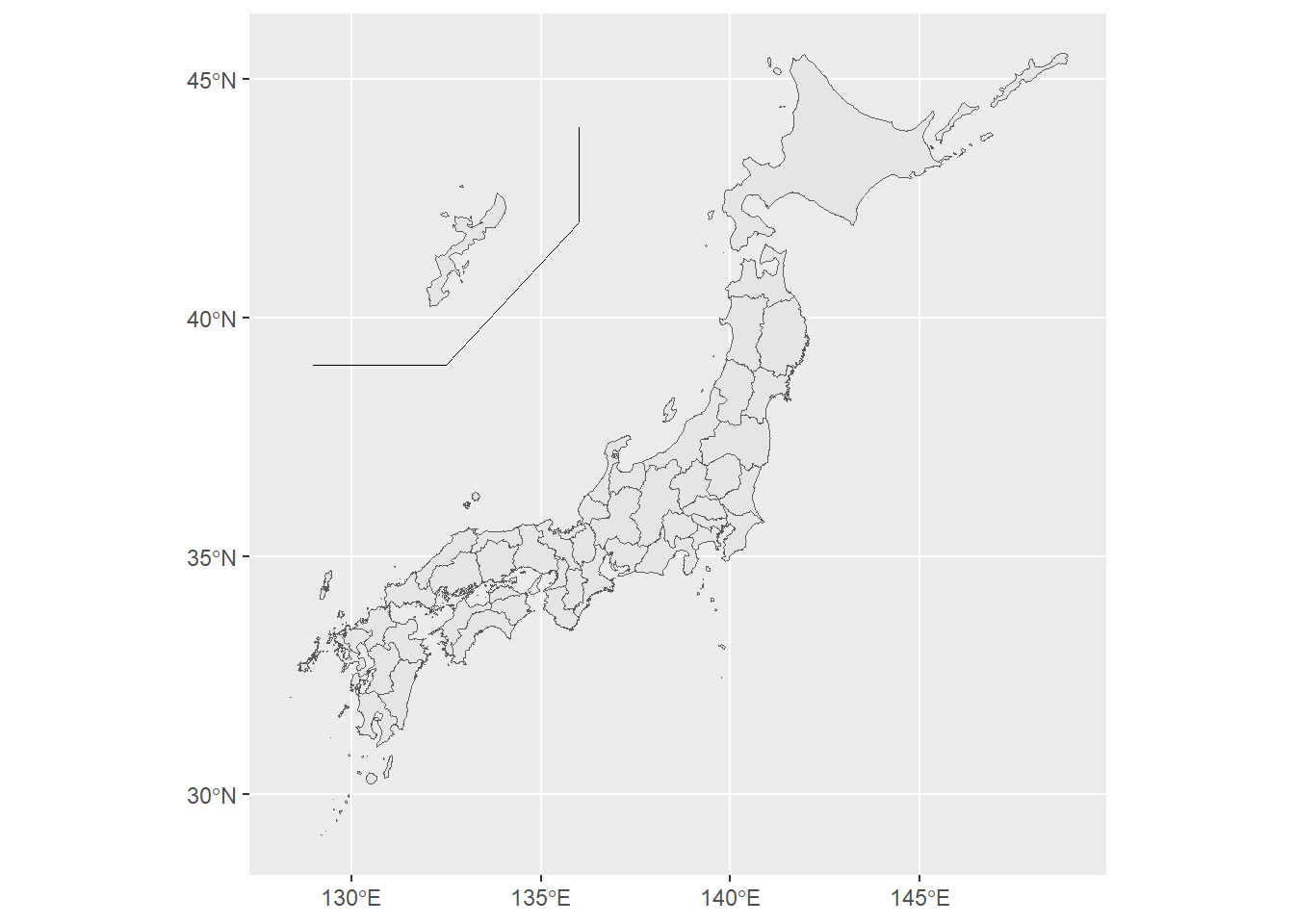

コロプレスマップ

datadf <- data.frame(prefID = simple_japanmap$prefID, value = simple_japanmap$prefID %>%
    as.numeric())
glimpse(datadf)

Rows: 47
Columns: 2
$ prefID <chr> "01", "02", "03", "04", "05", "06", "07", "08", "09", "10", "11…
$ value  <dbl> 1, 2, 3, 4, 5, 6, 7, 8, 9, 10, 11, 12, 13, 14, 15, 16, 17, 18, …

df <- left_join(simple_japanmap, datadf)
ggplot() + geom_sf(mapping = aes(fill = value), data = df) + func_add_segment_to_shp_map() + scale_fill_gradient2(low = "yellow", mid = "orange", high = "red", midpoint = 25) + theme(axis.title = element_blank())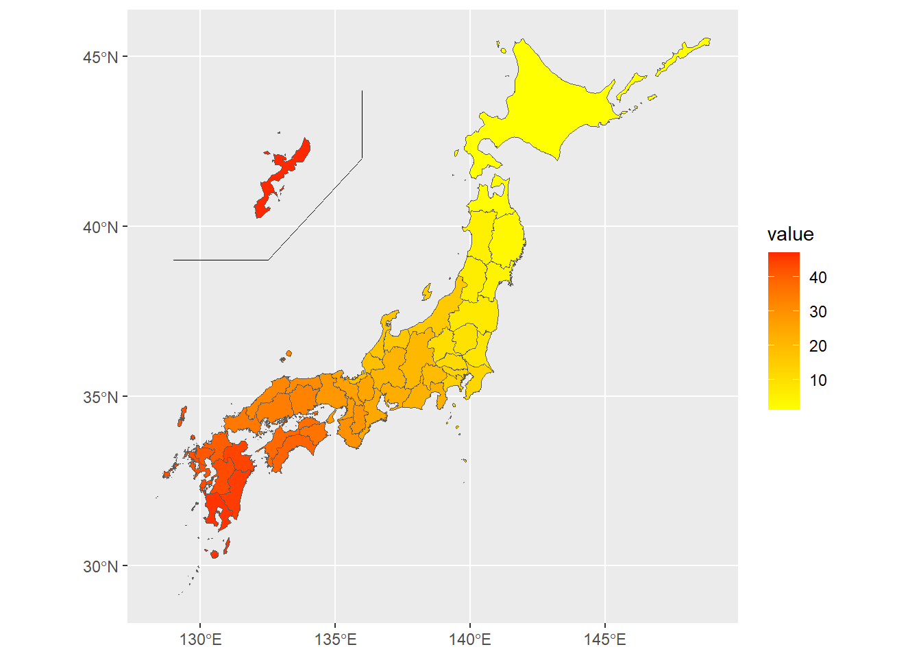

データソース

国土交通省:「国土数値情報ダウンロードサイト」行政区域第3.1版
https://nlftp.mlit.go.jp/ksj/gml/datalist/KsjTmplt-N03-2024.html

最終更新

Sys.time()

[1] "2024-04-11 16:57:10 JST"

R、Quarto、Package

R.Version()$version.string

[1] "R version 4.3.3 (2024-02-29 ucrt)"

quarto::quarto_version()

[1] '1.4.542'

packageVersion(pkg = "tidyverse")

[1] '2.0.0'

著者

アセット･マネジメント･コンサルティング株式会社 https://www.am-consulting.co.jp
法人概要 https://www.contact.am-consulting.co.jp/company-brochure/
代表取締役三竹道雄 https://www.contact.am-consulting.co.jp/mitake-michio/
公開コンテンツリスト https://www.am-consulting.co.jp/amc-all-contents.html
Charts https://www.am-consulting.co.jp/charts.html
法令検索 https://www.laws.am-consulting.co.jp/
SaECaNet https://www.saecanet.com/
twitter https://twitter.com/amc_corporation
youtube https://www.youtube.com/user/michiomitake
twilog https://twilog.togetter.com/amc_corporation
github https://github.com/am-consulting