library(ggplot2)
library(dplyr)
seed <- 20230321Rで回帰分析:一般化線形モデル(誤差構造:二項分布)
Rでデータサイエンス
一般化線形モデル(誤差構造:二項分布)
説明変数×2
# サンプルデータの作成
set.seed(seed)
b <- c(5, -3)  # 偏回帰係数
n <- 500  # サンプルサイズ
x1 <- runif(n = n)  # 説明変数
x2 <- runif(n = n)  # 説明変数
z <- (cbind(x1, x2) %*% b)
prob <- z %>%
    plogis()
# 目的変数
y <- sapply(X = prob, FUN = function(x) rbinom(n = 1, size = 1, prob = x))
data.frame(x1, x2, z, prob, y) %>%
    glimpse()
Rows: 500
Columns: 5
$ x1 <dbl> 0.78477723, 0.49618591, 0.96781807, 0.26996466, 0.95446996, 0.714…
$ x2 <dbl> 0.6128561478, 0.4846133357, 0.3128286593, 0.0191778555, 0.0003222…
$ z <dbl> 2.08531768, 1.02708956, 3.90060436, 1.29228974, 4.77138322, 3.349…
$ prob <dbl> 0.88946792, 0.73635126, 0.98017144, 0.78453450, 0.99160246, 0.966…
$ y <int> 1, 1, 1, 0, 1, 1, 0, 1, 1, 0, 1, 1, 1, 1, 1, 1, 0, 1, 0, 0, 1, 1,…ggplot(mapping = aes(x = prob)) + geom_histogram(binwidth = 0.1, closed = "left", boundary = 0, fill = "skyblue", col = "black") + theme_minimal()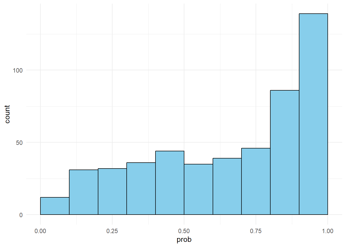
# ロジスティック回帰分析
result <- glm(formula = y ~ x1 + x2 - 1, family = binomial(link = "logit"))
result %>%
    summary()
Call:
glm(formula = y ~ x1 + x2 - 1, family = binomial(link = "logit"))

Coefficients:
   Estimate Std. Error z value            Pr(>|z|)
x1   5.2302     0.4664  11.213 <0.0000000000000002 ***
x2  -2.9798     0.3552  -8.389 <0.0000000000000002 ***
---
Signif. codes:  0 '***' 0.001 '**' 0.01 '*' 0.05 '.' 0.1 ' ' 1

(Dispersion parameter for binomial family taken to be 1)

    Null deviance: 693.15  on 500  degrees of freedom
Residual deviance: 433.18  on 498  degrees of freedom
AIC: 437.18

Number of Fisher Scoring iterations: 5confint(object = result, level = 0.95) 2.5 % 97.5 %
x1 4.361579 6.194014
x2 -3.704408 -2.309026# オッズ比の95%信頼区間
exp(confint(object = result, level = 0.95)) 2.5 % 97.5 %
x1 78.38081378 489.80803341
x2 0.02461478 0.09935801説明変数×1
# サンプルデータの作成
set.seed(seed)
b1 <- 8  # 回帰係数
b0 <- -2  # 切片
n <- 500  # サンプルサイズ
x <- runif(n = n, min = -1, max = 1)  # 説明変数
z <- x * b1 + b0
prob <- z %>%
    plogis()
# 目的変数
y <- sapply(X = prob, FUN = function(x) rbinom(n = 1, size = 1, prob = x))
data.frame(x, z, prob, y) %>%
    glimpse()
Rows: 500
Columns: 4
$ x <dbl> 0.569554451, -0.007628175, 0.935636137, -0.460070678, 0.908939929…
$ z <dbl> 2.5564356, -2.0610254, 5.4850891, -5.6805654, 5.2715194, 1.439349…
$ prob <dbl> 0.92800467655, 0.11294305765, 0.99586897072, 0.00340002923, 0.994…
$ y <int> 1, 0, 1, 0, 1, 1, 0, 0, 1, 0, 0, 0, 0, 1, 1, 0, 0, 1, 0, 0, 0, 1,…# ロジスティック回帰分析
result <- glm(formula = y ~ x, family = binomial(link = "logit"))
result %>%
summary()
Call:
glm(formula = y ~ x, family = binomial(link = "logit"))

Coefficients:
            Estimate Std. Error z value             Pr(>|z|)
(Intercept)  -1.8797     0.2590  -7.259    0.000000000000391 ***
x             7.9377     0.7862  10.097 < 0.0000000000000002 ***
---
Signif. codes:  0 '***' 0.001 '**' 0.01 '*' 0.05 '.' 0.1 ' ' 1

(Dispersion parameter for binomial family taken to be 1)

    Null deviance: 666.93  on 499  degrees of freedom
Residual deviance: 199.49  on 498  degrees of freedom
AIC: 203.49

Number of Fisher Scoring iterations: 7confint(object = result, level = 0.95) 2.5 % 97.5 %
(Intercept) -2.425126 -1.405209
x 6.528896 9.625312# プロット
g <- ggplot(data = data.frame(x, y), mapping = aes(x = x, y = y)) + geom_point() + geom_smooth(method = "glm", method.args = list(family = binomial(link = "logit")), se = F) + theme_minimal()
fun_prob <- function(z) {
exp(z)/(1 + exp(z))
}
g + stat_function(fun = function(x) fun_prob(z = (cbind(1, x) %*% coef(result))), color = "red", linewidth = 1, linetype = "dashed")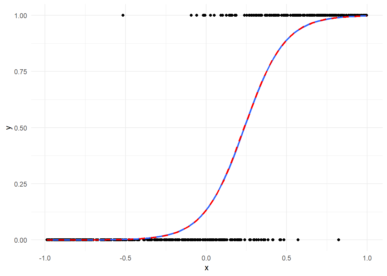
参考引用資料
最終更新
Sys.time()[1] "2024-03-31 05:35:21 JST"R、Quarto、Package
R.Version()$version.string[1] "R version 4.3.3 (2024-02-29 ucrt)"quarto::quarto_version()[1] '1.4.542'packageVersion(pkg = "tidyverse")[1] '2.0.0'