lapply(X = c("dplyr", "ggplot2", "knitr", "kableExtra"), require, character.only = T)Rで確率・統計:一般化線形モデルの信頼区間:誤差構造:二項分布、リンク関数:ロジット関数
Rでデータサイエンス
一般化線形モデルの信頼区間:誤差構造:二項分布、リンク関数:ロジット関数
サンプルデータ
# サンプルデータは mtcars を利用
mtcars %>%
    head()
mpg cyl disp hp drat wt qsec vs am gear carb
Mazda RX4 21.0 6 160 110 3.90 2.620 16.46 0 1 4 4
Mazda RX4 Wag 21.0 6 160 110 3.90 2.875 17.02 0 1 4 4
Datsun 710 22.8 4 108 93 3.85 2.320 18.61 1 1 4 1
Hornet 4 Drive 21.4 6 258 110 3.08 3.215 19.44 1 0 3 1
Hornet Sportabout 18.7 8 360 175 3.15 3.440 17.02 0 0 3 2
Valiant 18.1 6 225 105 2.76 3.460 20.22 1 0 3 1# 信頼水準は全て次の通り
cl <- 0.05
# 誤差構造を二項分布、リンク関数をロジット関数、説明変数をwt、目的変数をamとして一般化線形モデルでの回帰線を信頼区間付きで表示
link <- "logit"
point_size <- 0.7
g0 <- ggplot(data = mtcars, mapping = aes(x = wt, y = am)) + geom_point(size = point_size) + geom_smooth(method = "glm", method.args = list(family = binomial(link = link)), se = T, level = 1 - cl)
g0
# 以下で、青の回帰線とグレイの信頼区間の数値を確認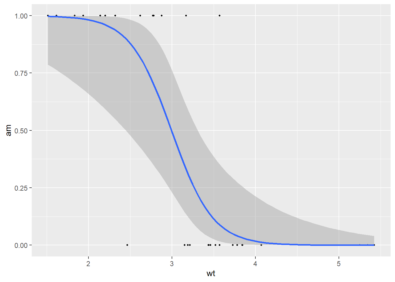
モデル作成
# 一般化線形モデルを作成
model <- glm(am ~ wt, data = mtcars, family = binomial(link = link))
model %>%
    summary
Call:
glm(formula = am ~ wt, family = binomial(link = link), data = mtcars)

Coefficients:
            Estimate Std. Error z value Pr(>|z|)
(Intercept)   12.040      4.510   2.670  0.00759 **
wt            -4.024      1.436  -2.801  0.00509 **
---
Signif. codes:  0 '***' 0.001 '**' 0.01 '*' 0.05 '.' 0.1 ' ' 1

(Dispersion parameter for binomial family taken to be 1)

    Null deviance: 43.230  on 31  degrees of freedom
Residual deviance: 19.176  on 30  degrees of freedom
AIC: 23.176

Number of Fisher Scoring iterations: 6confint(model, level = 1 - cl)
# 有意な係数が現れています。 2.5 % 97.5 %
(Intercept) 5.213795 23.628911
wt -7.698930 -1.833365信頼区間の算出
# サンプルデータ wt の最小値と最大値の間で説明変数 wt を100点用意
newdata <- data.frame(wt = seq(min(mtcars$wt), max(mtcars$wt), length = 100))
newdata %>%
    tail(6)
wt
95 5.226475
96 5.265980
97 5.305485
98 5.344990
99 5.384495
100 5.424000# それぞれの点で上記モデルによる目的変数の推定値を関数 predict により求める
# type = 'response'とすることで、回帰線の数値が直接取り出せますが、此処では線形予測での結果を返す
predict_result <- predict(object = model, newdata = newdata, type = "link", se.fit = T, level = 1 - cl)# 結果を上で作成しました説明変数100点と結合
# 線形予測で求めた目的変数の推定値
newdata$fit <- predict_result$fit
newdata$se <- predict_result$se.fit
newdata %>%
tail(6) wt fit se
95 5.226475 -8.990808 3.091054
96 5.265980 -9.149775 3.146799
97 5.305485 -9.308742 3.202579
98 5.344990 -9.467709 3.258392
99 5.384495 -9.626676 3.314237
100 5.424000 -9.785643 3.370112# 次の関数で線形予測の結果を目的変数amの期待値に変換
calc_p <- function(x) {
# ロジット関数の逆関数
p <- exp(x)/(1 + exp(x))
return(p)
}\[y = \textrm {log} \dfrac{p}{1-p},\quad e^y = \dfrac {p}{1-p},\quad p = e^y-e^yp,\quad e^y = p + e^yp = p\left(1+e^y\right),\quad p = \dfrac{e^y}{1+e^y}\]
# 推定された目的変数amは4列目
newdata$fit_logit <- newdata$fit %>%
    calc_p()
newdata %>%
    tail(6)
wt fit se fit_logit
95 5.226475 -8.990808 3.091054 0.00012453395
96 5.265980 -9.149775 3.146799 0.00010623244
97 5.305485 -9.308742 3.202579 0.00009062028
98 5.344990 -9.467709 3.258392 0.00007730234
99 5.384495 -9.626676 3.314237 0.00006594153
100 5.424000 -9.785643 3.370112 0.00005625028# 線形予測時点では正規分布を仮定している
cval <- qnorm(1 - cl/2)
cval[1] 1.959964# 上側、下側の信頼区間を求める
newdata$fit_logit_upper <- {
newdata$fit + cval * newdata$se
} %>%
calc_p()
newdata$fit_logit_lower <- {
newdata$fit - cval * newdata$se
} %>%
calc_p()
newdata %>%
tail(6) wt fit se fit_logit fit_logit_upper fit_logit_lower
95 5.226475 -8.990808 3.091054 0.00012453395 0.05057237 0.00000029122733
96 5.265980 -9.149775 3.146799 0.00010623244 0.04823823 0.00000022271192
97 5.305485 -9.308742 3.202579 0.00009062028 0.04600961 0.00000017030400
98 5.344990 -9.467709 3.258392 0.00007730234 0.04388196 0.00000013022005
99 5.384495 -9.626676 3.314237 0.00006594153 0.04185087 0.00000009956437
100 5.424000 -9.785643 3.370112 0.00005625028 0.03991212 0.00000007612098# ggplotで作成したチャートにそれぞれの点を重ねます。
# 赤点が求めた数値です。
# 回帰線
g1 <- g0 + geom_point(data = newdata, mapping = aes(x = wt, y = fit_logit), color = "red", size = point_size)
# 信頼区間上側
g2 <- g1 + geom_point(data = newdata, mapping = aes(x = wt, y = fit_logit_upper), color = "red", size = point_size)
# 信頼区間下側
g <- g2 + geom_point(data = newdata, mapping = aes(x = wt, y = fit_logit_lower), color = "red", size = point_size)
g
# 全て重なります。
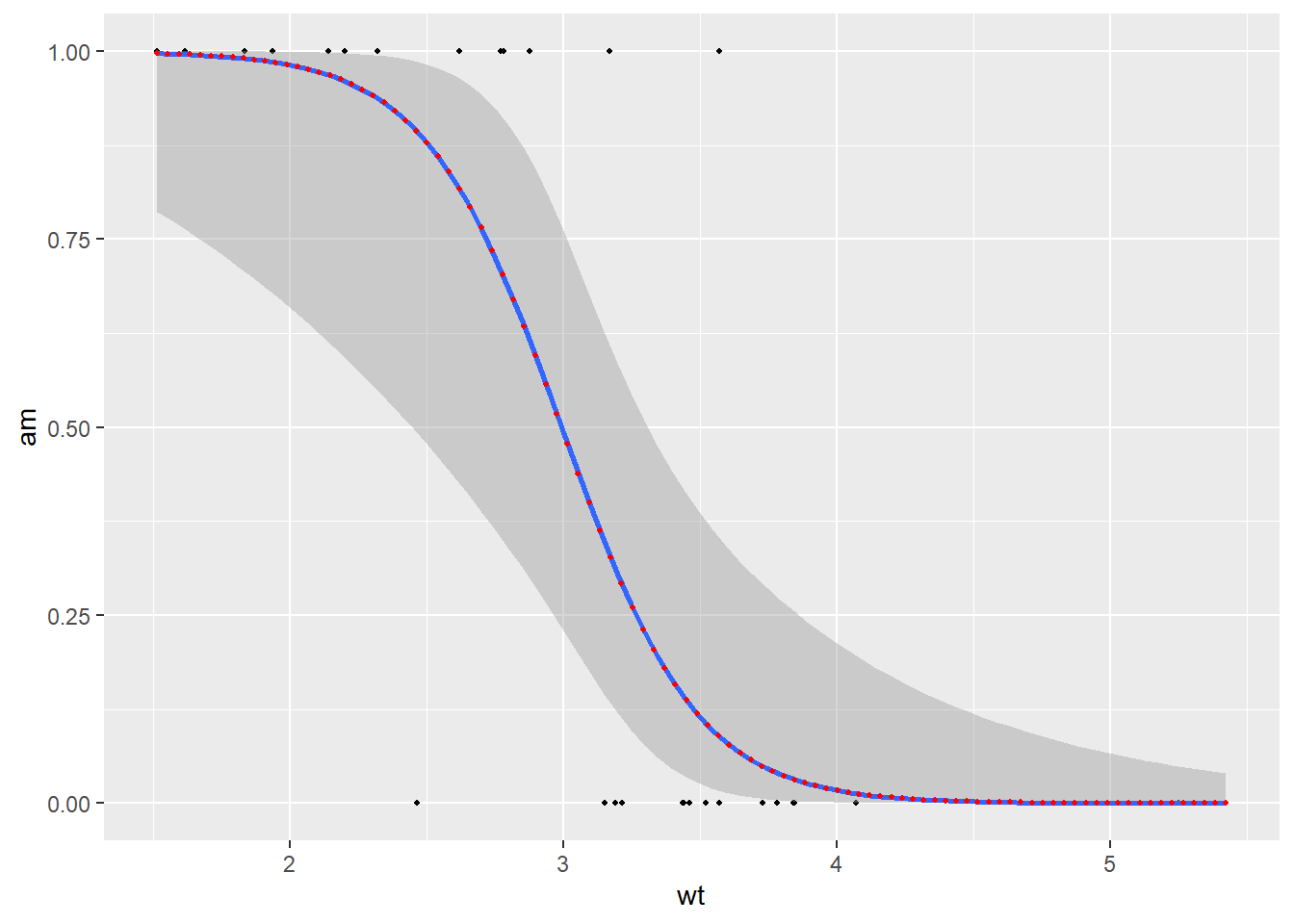
# なお関数predictを用いずとも回帰線の数値は以下の通りに取り出せます
liner_y <- model$coefficients[2] * newdata$wt + model$coefficients[1]
y_hat <- exp(liner_y)/(1 + exp(liner_y))
g0 + geom_point(data = newdata, mapping = aes(x = newdata$wt, y = y_hat), color = "red", size = point_size)
# こちらも回帰線が重なります。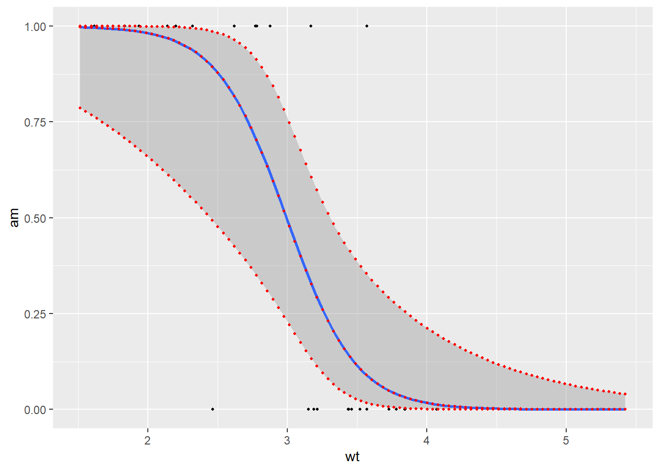
参考引用資料
- https://www.slideshare.net/logics-of-blue/2-3glm
- https://stats.biopapyrus.jp/glm/logit-regression.html
- http://cse.naro.affrc.go.jp/yamamura/Images/kenshuu_slide_glm_2017.pdf
- http://faculty.washington.edu/eliezg/teaching/StatR201/VisualizingPredictions.html
- https://jp.mathworks.com/help/stats/examples/fitting-data-with-generalized-linear-models.html
- http://faculty.washington.edu/eliezg/teaching/StatR201/VisualizingPredictions.html
- https://www.jstage.jst.go.jp/article/weed/55/4/55_4_268/_pdf
- https://fromthebottomoftheheap.net/2018/12/10/confidence-intervals-for-glms/
- https://stats.stackexchange.com/questions/41074/prediction-with-ci-predict-glm-doesnt-have-interval-option
- https://stackoverflow.com/questions/14423325/confidence-intervals-for-predictions-from-logistic-regression
- https://stackoverflow.com/questions/48331543/transform-family-link-functions-in-glm-predictions-in-r
最終更新
Sys.time()[1] "2024-04-16 10:24:46 JST"R、Quarto、Package
R.Version()$version.string[1] "R version 4.3.3 (2024-02-29 ucrt)"quarto::quarto_version()[1] '1.4.553'packageVersion(pkg = "tidyverse")[1] '2.0.0'