一般化線形モデルの信頼区間:誤差構造:ガンマ分布、リンク関数:ログ関数
サンプルデータ
# サンプルデータは mtcars を利用
mtcars %>%
    tail()
                mpg cyl  disp  hp drat    wt qsec vs am gear carb
Porsche 914-2  26.0   4 120.3  91 4.43 2.140 16.7  0  1    5    2
Lotus Europa   30.4   4  95.1 113 3.77 1.513 16.9  1  1    5    2
Ford Pantera L 15.8   8 351.0 264 4.22 3.170 14.5  0  1    5    4
Ferrari Dino   19.7   6 145.0 175 3.62 2.770 15.5  0  1    5    6
Maserati Bora  15.0   8 301.0 335 3.54 3.570 14.6  0  1    5    8
Volvo 142E     21.4   4 121.0 109 4.11 2.780 18.6  1  1    4    2
# 以降、信頼水準は全て次の通り
cl <- 0.05
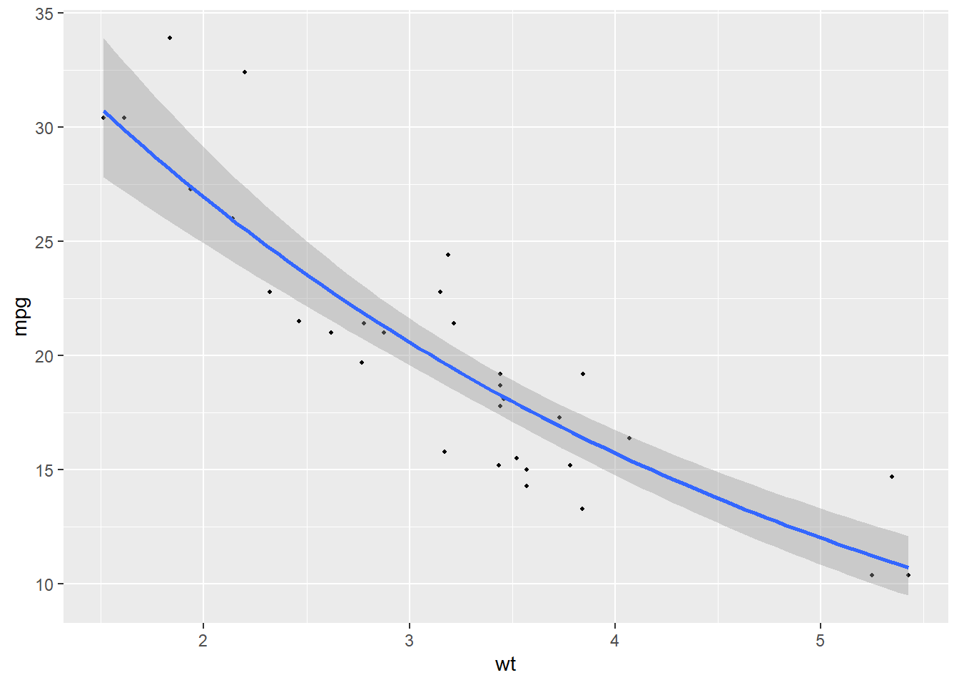
# 誤差構造をガンマ分布、リンク関数をログ関数とし、説明変数をwt、目的変数をmpgとして一般化線形モデルでの回帰線を信頼区間付きで表示
link <- "log"
point_size <- 0.7
g0 <- ggplot(data = mtcars, mapping = aes(x = wt, y = mpg)) + geom_point(size = point_size) + geom_smooth(method = "glm", method.args = list(family = Gamma(link = link)), se = T, level = 1 - cl)
g0
# 以下で、青の回帰線とグレイの信頼区間の数値を確認
モデル作成
# 一般化線形モデルを作成
model <- glm(formula = mpg ~ wt, data = mtcars, family = Gamma(link = link))
model %>%
    summary
Call:
glm(formula = mpg ~ wt, family = Gamma(link = link), data = mtcars)

Coefficients:
            Estimate Std. Error t value             Pr(>|t|)
(Intercept)  3.83186    0.08647   44.31 < 0.0000000000000002 ***
wt          -0.26901    0.02575  -10.45      0.0000000000163 ***
---
Signif. codes:  0 '***' 0.001 '**' 0.01 '*' 0.05 '.' 0.1 ' ' 1

(Dispersion parameter for Gamma family taken to be 0.01967651)

    Null deviance: 2.73529  on 31  degrees of freedom
Residual deviance: 0.56667  on 30  degrees of freedom
AIC: 157.11

Number of Fisher Scoring iterations: 4
信頼区間の算出
confint(model, level = 1 - cl)
# 有意な係数が現れています(*devianceは無視)。
                 2.5 %     97.5 %
(Intercept)  3.6668503  3.9980063
wt          -0.3180287 -0.2196311
# サンプルデータwtの最小値と最大値の間で説明変数wtを100点用意
newdata <- data.frame(wt = seq(min(mtcars$wt), max(mtcars$wt), length = 100))
newdata %>%
    tail()
          wt
95  5.226475
96  5.265980
97  5.305485
98  5.344990
99  5.384495
100 5.424000
# それぞれの点で上記モデルによる目的変数の推定値を関数predictにより求める
# type = 'response'とすることで回帰線の数値が直接取り出せますが此処では線形予測での結果を返す
predict_result <- predict(object = model, newdata = newdata, type = "link", se.fit = T, level = 1 - cl)
# 結果を上で作成しました説明変数100点と結合
# 線形予測で求めた目的変数の推定値
newdata$fit <- predict_result$fit
newdata$se <- predict_result$se.fit
newdata %>%
    tail()
          wt      fit         se
95  5.226475 2.425858 0.05737023
96  5.265980 2.415230 0.05828916
97  5.305485 2.404603 0.05921130
98  5.344990 2.393975 0.06013651
99  5.384495 2.383348 0.06106464
100 5.424000 2.372721 0.06199557
# 次の関数で線形予測の結果を目的変数mpgの期待値に変換
calc_y_hat <- function(x) {
    y_hat <- exp(x)
    return(y_hat)
}
\[\textrm{log}Y = aX+b,\quad Y = e^{aX+b}\]
# 推定された目的変数mpgは4列目
newdata$fit_log <- newdata$fit %>%
    calc_y_hat()
newdata %>%
    tail()
          wt      fit         se  fit_log
95  5.226475 2.425858 0.05737023 11.31193
96  5.265980 2.415230 0.05828916 11.19235
97  5.305485 2.404603 0.05921130 11.07403
98  5.344990 2.393975 0.06013651 10.95697
99  5.384495 2.383348 0.06106464 10.84114
100 5.424000 2.372721 0.06199557 10.72654
# 線形予測時点では正規分布を仮定している
cval <- qnorm(1 - cl/2)
cval
# 上側、下側の信頼区間を求める
newdata$fit_log_upper <- {
    newdata$fit + cval * newdata$se
} %>%
    calc_y_hat()
newdata$fit_log_lower <- {
    newdata$fit - cval * newdata$se
} %>%
    calc_y_hat()
newdata %>%
    tail()
          wt      fit         se  fit_log fit_log_upper fit_log_lower
95  5.226475 2.425858 0.05737023 11.31193      12.65815     10.108880
96  5.265980 2.415230 0.05828916 11.19235      12.54692      9.984019
97  5.305485 2.404603 0.05921130 11.07403      12.43674      9.860638
98  5.344990 2.393975 0.06013651 10.95697      12.32760      9.738724
99  5.384495 2.383348 0.06106464 10.84114      12.21949      9.618262
100 5.424000 2.372721 0.06199557 10.72654      12.11240      9.499237
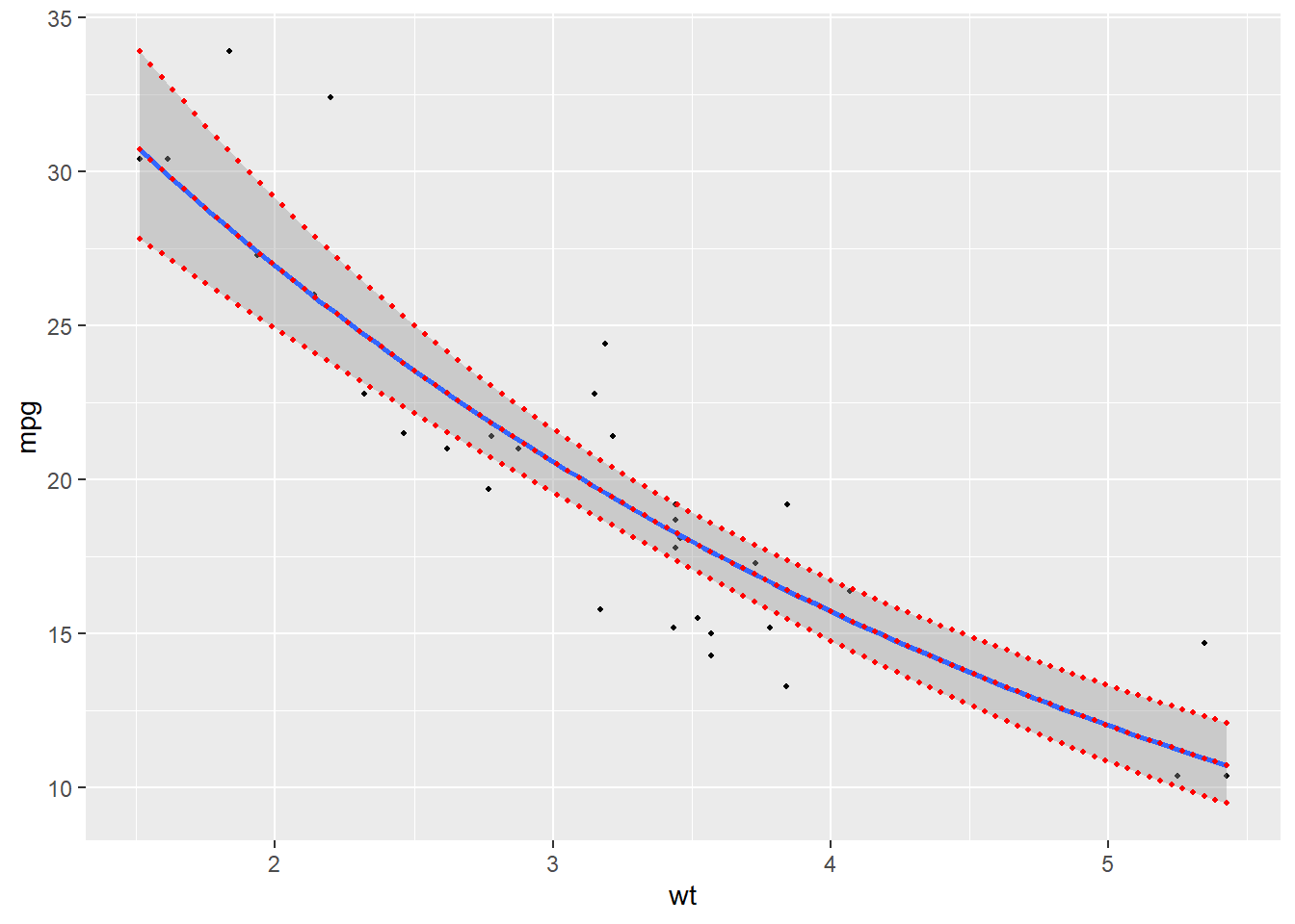
# ggplotで作成したチャートにそれぞれの点を重ねます。
# 赤点が求めた数値です。
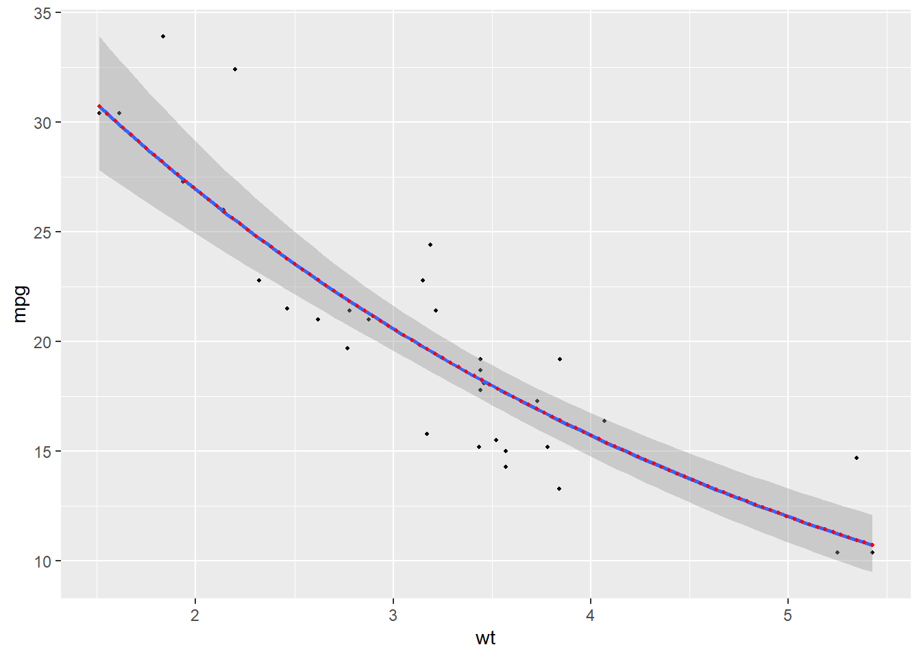
# 回帰線
g1 <- g0 + geom_point(data = newdata, mapping = aes(x = newdata$wt, y = newdata$fit_log), color = "red", size = point_size)
# 信頼区間上側
g2 <- g1 + geom_point(data = newdata, mapping = aes(x = wt, y = fit_log_upper), color = "red", size = point_size)
# 信頼区間下側
g <- g2 + geom_point(data = newdata, mapping = aes(x = wt, y = fit_log_lower), color = "red", size = point_size)
g
# 全て重なります。
# なお関数predictを用いずとも回帰線の数値は以下の通りに取り出せます。
y_hat <- {
model$coefficients[2] * newdata$wt + model$coefficients[1]
} %>%
exp()
g0 + geom_point(data = newdata, mapping = aes(x = newdata$wt, y = y_hat), color = "red", size = point_size)
# こちらも回帰線が重なります。
最終更新
[1] "2024-04-17 04:56:55 JST"
R、Quarto、Package
R.Version()$version.string
[1] "R version 4.3.3 (2024-02-29 ucrt)"
packageVersion(pkg = "tidyverse")
著者
Figure 1:
Figure 2:
Figure 3: