library(dplyr)
library(ggplot2)
func_sim_ar <- function(p,n,a_min,a_max,method = 'recursive'){
  # recursive:再帰的
  # 係数
  a <- seq(a_min,a_max,0.001) %>% sample(size = p);a
  # 撹乱項
  epsilon <- rnorm(n - p);epsilon
  # 時系列の初期値
  x0 <- rnorm(p);x0
  # AR
  x <- c(x0,stats::filter(x = epsilon,filter = a,method = method,init = rev(x0)))
  return(list(a = a,epsilon = epsilon,x = x,x0 = x0))
}Rで時系列分析:自己回帰モデル AR(p)
Rでデータサイエンス
AR(p)
\(p\)次の自己回帰モデル
\[y_t=c+\phi_1y_{t-1}+\phi_2y_{t-2}+\cdots+\phi_py_{t-p}+\epsilon_t\quad0<\phi<1\]
AR(1)\(y_t=\phi y_{t-1}+\epsilon_t\)に1期前の\(y_{t-1}=\phi y_{t-2}+\epsilon_{t-1}\)を代入すると\[y_t=\phi^2 y_{t-2}+\phi\epsilon_{t-1}+\epsilon_t\]この代入操作を繰り返すと\[y_t=\phi^py_{t-p}+\displaystyle\sum_{s=0}^{p-1}\phi^s\epsilon_{t-s}\]が得られる。ここで\(p\rightarrow\infty,\,0<\phi<1\)とすると\[y_t=\displaystyle\sum_{s=0}^\infty \phi^s\epsilon_{t-s}=\epsilon_t+\phi\epsilon_{t-1}+\phi^2\epsilon_{t-2}+\cdots\]つまり\(p\rightarrow\infty,0<\phi<1\)の下,ARモデルはイノベーション(撹乱項,\(\epsilon\))の無限加重和で表現できる.
参考引用資料
- 加藤久和(2012),『gretlで計量経済分析』,日本評論社,pp.134-136
ARモデルのシミュレーション
# ラグ次数
p <- 2
# サンプルサイズ
n <- 100
# 係数の下限
a_min <- -0.5
# 係数の上限
a_max <- 0.5
result <- func_sim_ar(p = p,n = n,a_min = a_min,a_max = a_max)
a <- result$a#;a
ep <- result$epsilon
x <- result$x
x0 <- result$x0#;x0
df <- data.frame(n = seq(length(x)),x = x)
colnames(df)[2] <- paste0('a = ',paste0(a,collapse = ',') )#;head(df)
ggplot(mapping = aes(x = df[,1],y = df[,2])) + geom_line(size = 0.1) + geom_point(size = 1) +
  theme(axis.title = element_blank()) + labs(title = colnames(df)[2])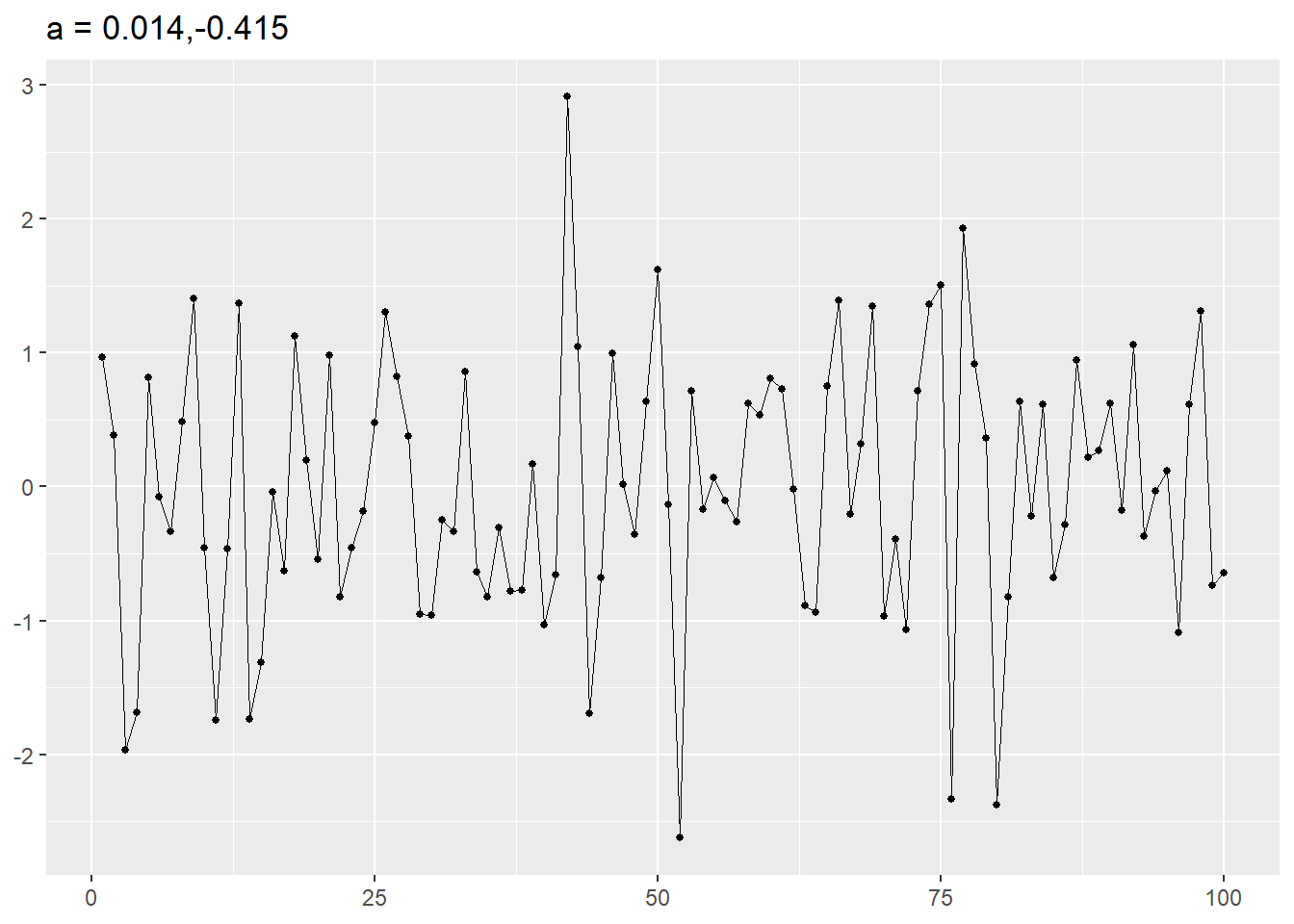
# 確認
a[1]*x[2] + a[2]*x[1] + ep[1]
x[3]
[1] -1.963251
[1] -1.963251# 確認
a[1]*x[12] + a[2]*x[11] + ep[11]
x[13][1] 1.366318
[1] 1.366318# 確認
a[1]*x[99] + a[2]*x[98] + ep[98]
x[100][1] -0.6409794
[1] -0.6409794参考引用資料
最終更新
Sys.time()[1] "2024-04-26 08:19:53 JST"R、Quarto、Package
R.Version()$version.string[1] "R version 4.3.3 (2024-02-29 ucrt)"quarto::quarto_version()[1] '1.4.553'packageVersion(pkg = "tidyverse")[1] '2.0.0'