Analysis
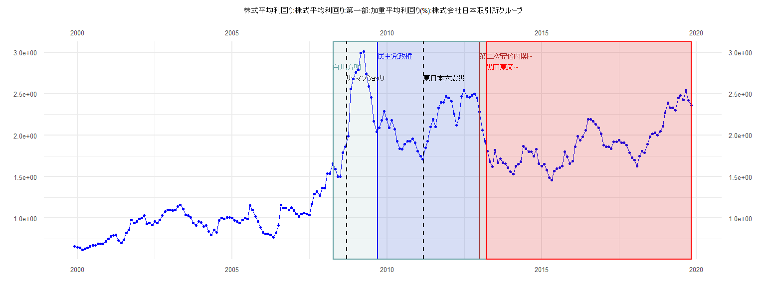
[1] "株式平均利回り:株式平均利回り:第一部:加重平均利回り(%):株式会社日本取引所グループ"
      Jan  Feb  Mar  Apr  May  Jun  Jul  Aug  Sep  Oct  Nov  Dec
1999                                                   0.66 0.65
2000 0.64 0.62 0.63 0.64 0.66 0.67 0.67 0.69 0.69 0.69 0.72 0.75
2001 0.78 0.79 0.80 0.73 0.70 0.74 0.82 0.86 0.98 0.94 0.96 0.99
2002 1.00 1.03 0.93 0.94 0.92 0.96 0.94 0.98 1.03 1.08 1.10 1.10
2003 1.09 1.10 1.14 1.16 1.11 1.04 1.03 1.01 0.94 0.91 0.96 0.95
2004 0.90 0.91 0.84 0.80 0.86 0.83 0.97 1.00 0.99 1.01 1.01 1.00
2005 0.97 0.96 0.94 0.98 1.00 0.99 1.15 1.10 1.02 0.96 0.89 0.83
2006 0.81 0.81 0.80 0.77 0.82 0.91 1.16 1.12 1.12 1.10 1.13 1.09
2007 1.05 1.02 1.05 1.06 1.05 1.04 1.17 1.29 1.32 1.27 1.36 1.36
2008 1.54 1.54 1.66 1.59 1.50 1.50 1.79 1.86 1.99 2.56 2.68 2.76
2009 2.79 2.99 3.01 2.74 2.59 2.46 2.17 2.04 2.09 2.18 2.29 2.19
2010 2.09 2.18 2.07 1.93 1.84 1.83 1.89 1.93 1.93 1.96 1.91 1.81
2011 1.75 1.71 1.85 1.93 2.10 2.19 2.10 2.33 2.40 2.40 2.47 2.45
2012 2.41 2.26 2.12 2.21 2.47 2.54 2.47 2.46 2.48 2.50 2.45 2.28
2013 2.06 1.93 1.81 1.68 1.62 1.82 1.67 1.72 1.67 1.66 1.61 1.56
2014 1.53 1.63 1.65 1.68 1.87 1.84 1.80 1.80 1.75 1.83 1.66 1.63
2015 1.65 1.58 1.49 1.46 1.57 1.60 1.61 1.63 1.80 1.74 1.66 1.69
2016 1.86 1.99 1.94 1.98 2.06 2.19 2.19 2.17 2.13 2.09 2.02 1.88
2017 1.86 1.86 1.84 1.92 1.92 1.94 1.91 1.91 1.88 1.79 1.73 1.70
2018 1.63 1.75 1.81 1.79 1.89 1.98 2.02 2.03 2.00 2.05 2.11 2.27
2019 2.39 2.33 2.33 2.30 2.45 2.48 2.43 2.54 2.42 2.36
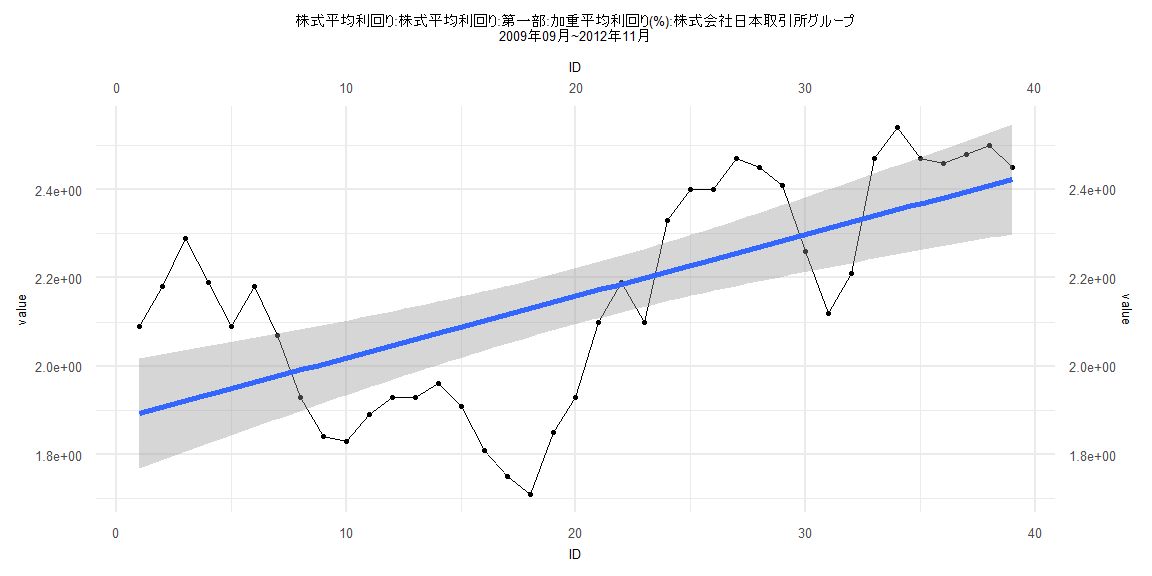
Call:
lm(formula = value ~ ID)

Residuals:
     Min       1Q   Median       3Q      Max
-0.42032 -0.13666  0.02687  0.14954  0.36883

Coefficients:
            Estimate Std. Error t value             Pr(>|t|)
(Intercept) 1.879339   0.063540  29.577 < 0.0000000000000002 ***
ID          0.013943   0.002769   5.036            0.0000126 ***
---
Signif. codes:  0 '***' 0.001 '**' 0.01 '*' 0.05 '.' 0.1 ' ' 1

Residual standard error: 0.1946 on 37 degrees of freedom
Multiple R-squared:  0.4067,    Adjusted R-squared:  0.3906
F-statistic: 25.36 on 1 and 37 DF,  p-value: 0.00001262


    Two-sample Kolmogorov-Smirnov test

data:  lm_residuals and rnorm(n = length(lm_residuals), mean = 0, sd = sd(lm_residuals))
D = 0.28205, p-value = 0.08974
alternative hypothesis: two-sided


    Durbin-Watson test

data:  value ~ ID
DW = 0.26846, p-value = 0.000000000000008286
alternative hypothesis: true autocorrelation is greater than 0


    studentized Breusch-Pagan test

data:  value ~ ID
BP = 4.7625, df = 1, p-value = 0.02909


    Box-Ljung test

data:  lm_residuals
X-squared = 30.524, df = 1, p-value = 0.00000003297
Call:
lm(formula = value ~ ID)

Residuals:
     Min       1Q   Median       3Q      Max
-0.40633 -0.13026 -0.04037  0.15739  0.67198

Coefficients:
             Estimate Std. Error t value             Pr(>|t|)
(Intercept) 1.6009991  0.0447650  35.765 < 0.0000000000000002 ***
ID          0.0070215  0.0009258   7.584      0.0000000000492 ***
---
Signif. codes:  0 '***' 0.001 '**' 0.01 '*' 0.05 '.' 0.1 ' ' 1

Residual standard error: 0.2021 on 81 degrees of freedom
Multiple R-squared:  0.4153,    Adjusted R-squared:  0.408
F-statistic: 57.52 on 1 and 81 DF,  p-value: 0.00000000004924


    Two-sample Kolmogorov-Smirnov test

data:  lm_residuals and rnorm(n = length(lm_residuals), mean = 0, sd = sd(lm_residuals))
D = 0.072289, p-value = 0.9829
alternative hypothesis: two-sided


    Durbin-Watson test

data:  value ~ ID
DW = 0.18343, p-value < 0.00000000000000022
alternative hypothesis: true autocorrelation is greater than 0


    studentized Breusch-Pagan test

data:  value ~ ID
BP = 0.0087354, df = 1, p-value = 0.9255


    Box-Ljung test

data:  lm_residuals
X-squared = 60.034, df = 1, p-value = 0.000000000000009326
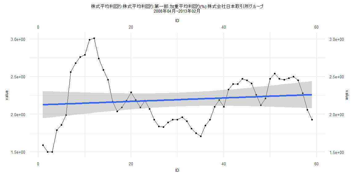
Call:
lm(formula = value ~ ID)

Residuals:
     Min       1Q   Median       3Q      Max
-0.63197 -0.27041 -0.02499  0.22310  0.85728

Coefficients:
            Estimate Std. Error t value            Pr(>|t|)
(Intercept) 2.125050   0.092123  23.068 <0.0000000000000002 ***
ID          0.002306   0.002671   0.864               0.391
---
Signif. codes:  0 '***' 0.001 '**' 0.01 '*' 0.05 '.' 0.1 ' ' 1

Residual standard error: 0.3493 on 57 degrees of freedom
Multiple R-squared:  0.01292,   Adjusted R-squared:  -0.004402
F-statistic: 0.7458 on 1 and 57 DF,  p-value: 0.3914


    Two-sample Kolmogorov-Smirnov test

data:  lm_residuals and rnorm(n = length(lm_residuals), mean = 0, sd = sd(lm_residuals))
D = 0.15254, p-value = 0.5021
alternative hypothesis: two-sided


    Durbin-Watson test

data:  value ~ ID
DW = 0.17088, p-value < 0.00000000000000022
alternative hypothesis: true autocorrelation is greater than 0


    studentized Breusch-Pagan test

data:  value ~ ID
BP = 15.023, df = 1, p-value = 0.0001062


    Box-Ljung test

data:  lm_residuals
X-squared = 48.701, df = 1, p-value = 0.000000000002981
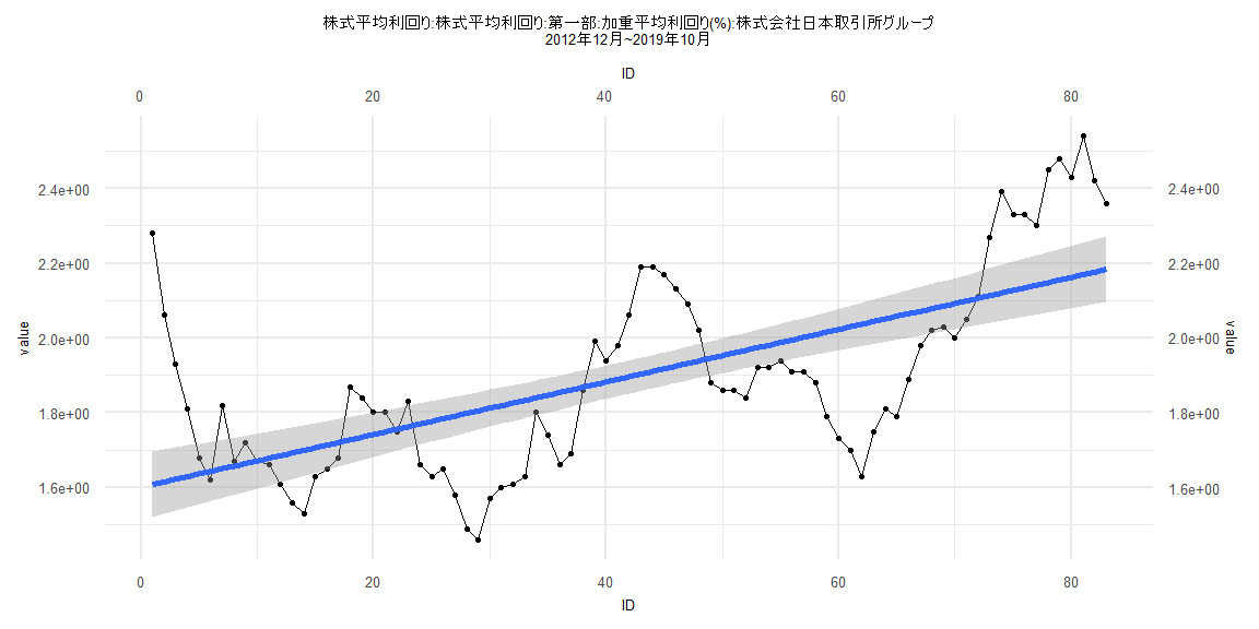
Call:
lm(formula = value ~ ID)

Residuals:
    Min      1Q  Median      3Q     Max
-0.4143 -0.1107 -0.0160  0.1346  0.3358

Coefficients:
             Estimate Std. Error t value             Pr(>|t|)
(Intercept) 1.5477690  0.0400436  38.652 < 0.0000000000000002 ***
ID          0.0084162  0.0008589   9.799  0.00000000000000308 ***
---
Signif. codes:  0 '***' 0.001 '**' 0.01 '*' 0.05 '.' 0.1 ' ' 1

Residual standard error: 0.1774 on 78 degrees of freedom
Multiple R-squared:  0.5518,    Adjusted R-squared:  0.546
F-statistic: 96.01 on 1 and 78 DF,  p-value: 0.000000000000003079


    Two-sample Kolmogorov-Smirnov test

data:  lm_residuals and rnorm(n = length(lm_residuals), mean = 0, sd = sd(lm_residuals))
D = 0.1375, p-value = 0.4383
alternative hypothesis: two-sided


    Durbin-Watson test

data:  value ~ ID
DW = 0.212, p-value < 0.00000000000000022
alternative hypothesis: true autocorrelation is greater than 0


    studentized Breusch-Pagan test

data:  value ~ ID
BP = 7.5914, df = 1, p-value = 0.005865


    Box-Ljung test

data:  lm_residuals
X-squared = 63.859, df = 1, p-value = 0.000000000000001332