Analysis
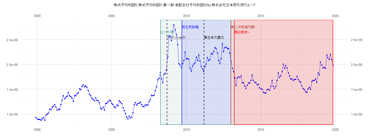
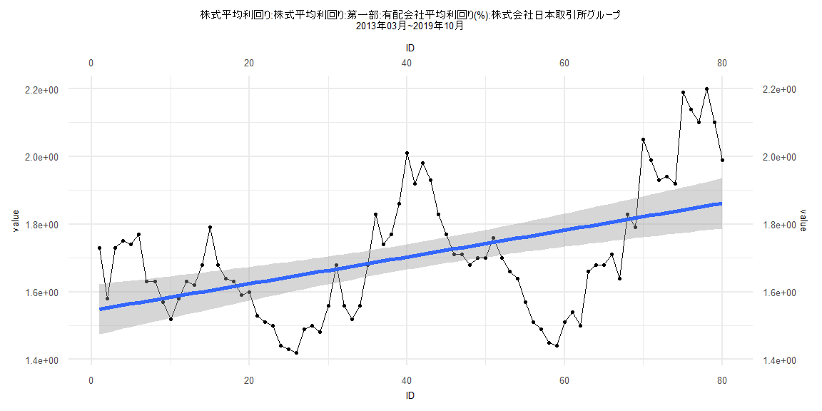
[1] "株式平均利回り:株式平均利回り:第一部:有配会社平均利回り(%):株式会社日本取引所グループ"
      Jan  Feb  Mar  Apr  May  Jun  Jul  Aug  Sep  Oct  Nov  Dec
1999                                                   0.93 0.90
2000 0.89 0.89 0.88 0.90 0.93 0.88 0.98 1.00 1.02 1.10 1.09 1.14
2001 1.16 1.19 1.15 1.08 1.10 1.09 1.19 1.28 1.37 1.31 1.34 1.36
2002 1.44 1.37 1.35 1.32 1.26 1.37 1.37 1.41 1.43 1.51 1.49 1.56
2003 1.59 1.55 1.57 1.54 1.47 1.40 1.37 1.32 1.30 1.27 1.33 1.28
2004 1.27 1.23 1.12 1.10 1.14 1.08 1.21 1.22 1.25 1.28 1.27 1.21
2005 1.19 1.15 1.13 1.18 1.17 1.27 1.24 1.21 1.13 1.07 1.01 0.94
2006 0.90 0.96 0.92 0.94 1.03 1.19 1.23 1.18 1.21 1.22 1.24 1.19
2007 1.16 1.15 1.18 1.18 1.18 1.25 1.29 1.38 1.37 1.38 1.47 1.55
2008 1.69 1.72 1.84 1.71 1.63 1.80 1.82 1.89 2.16 2.58 2.57 2.48
2009 2.66 2.80 2.70 2.60 2.40 2.02 1.99 1.94 2.02 2.08 2.25 2.11
2010 2.12 2.11 1.92 1.87 1.97 2.01 2.03 2.15 2.08 2.19 2.07 1.96
2011 1.91 1.86 1.96 2.01 2.14 2.08 2.10 2.22 2.21 2.26 2.34 2.32
2012 2.23 2.08 2.02 2.12 2.42 2.26 2.34 2.35 2.32 2.32 2.23 2.07
2013 1.92 1.86 1.73 1.58 1.73 1.75 1.74 1.77 1.63 1.63 1.57 1.52
2014 1.58 1.63 1.62 1.68 1.79 1.68 1.64 1.63 1.59 1.60 1.53 1.51
2015 1.50 1.44 1.43 1.42 1.49 1.50 1.48 1.56 1.68 1.56 1.52 1.56
2016 1.68 1.83 1.74 1.77 1.86 2.01 1.92 1.98 1.93 1.83 1.77 1.71
2017 1.71 1.68 1.70 1.70 1.76 1.70 1.66 1.64 1.57 1.51 1.49 1.45
2018 1.44 1.51 1.54 1.50 1.66 1.68 1.68 1.71 1.64 1.83 1.79 2.05
2019 1.99 1.93 1.94 1.92 2.19 2.14 2.10 2.20 2.10 1.99
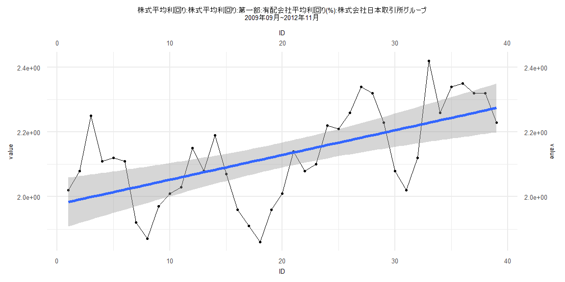
Call:
lm(formula = value ~ ID)

Residuals:
     Min       1Q   Median       3Q      Max
-0.25392 -0.08806  0.02359  0.08826  0.25092

Coefficients:
            Estimate Std. Error t value             Pr(>|t|)
(Intercept) 1.976113   0.038751  50.996 < 0.0000000000000002 ***
ID          0.007656   0.001689   4.534            0.0000589 ***
---
Signif. codes:  0 '***' 0.001 '**' 0.01 '*' 0.05 '.' 0.1 ' ' 1

Residual standard error: 0.1187 on 37 degrees of freedom
Multiple R-squared:  0.3572,    Adjusted R-squared:  0.3398
F-statistic: 20.56 on 1 and 37 DF,  p-value: 0.0000589


    Two-sample Kolmogorov-Smirnov test

data:  lm_residuals and rnorm(n = length(lm_residuals), mean = 0, sd = sd(lm_residuals))
D = 0.20513, p-value = 0.3888
alternative hypothesis: two-sided


    Durbin-Watson test

data:  value ~ ID
DW = 0.7624, p-value = 0.000002439
alternative hypothesis: true autocorrelation is greater than 0


    studentized Breusch-Pagan test

data:  value ~ ID
BP = 0.41919, df = 1, p-value = 0.5173


    Box-Ljung test

data:  lm_residuals
X-squared = 15.948, df = 1, p-value = 0.00006512
Call:
lm(formula = value ~ ID)

Residuals:
     Min       1Q   Median       3Q      Max
-0.33238 -0.12935 -0.02215  0.12614  0.47613

Coefficients:
             Estimate Std. Error t value             Pr(>|t|)
(Intercept) 1.5909462  0.0401004  39.674 < 0.0000000000000002 ***
ID          0.0029264  0.0008293   3.529             0.000692 ***
---
Signif. codes:  0 '***' 0.001 '**' 0.01 '*' 0.05 '.' 0.1 ' ' 1

Residual standard error: 0.181 on 81 degrees of freedom
Multiple R-squared:  0.1332,    Adjusted R-squared:  0.1225
F-statistic: 12.45 on 1 and 81 DF,  p-value: 0.0006915


    Two-sample Kolmogorov-Smirnov test

data:  lm_residuals and rnorm(n = length(lm_residuals), mean = 0, sd = sd(lm_residuals))
D = 0.13253, p-value = 0.4619
alternative hypothesis: two-sided


    Durbin-Watson test

data:  value ~ ID
DW = 0.22492, p-value < 0.00000000000000022
alternative hypothesis: true autocorrelation is greater than 0


    studentized Breusch-Pagan test

data:  value ~ ID
BP = 2.5078, df = 1, p-value = 0.1133


    Box-Ljung test

data:  lm_residuals
X-squared = 60.742, df = 1, p-value = 0.00000000000000655
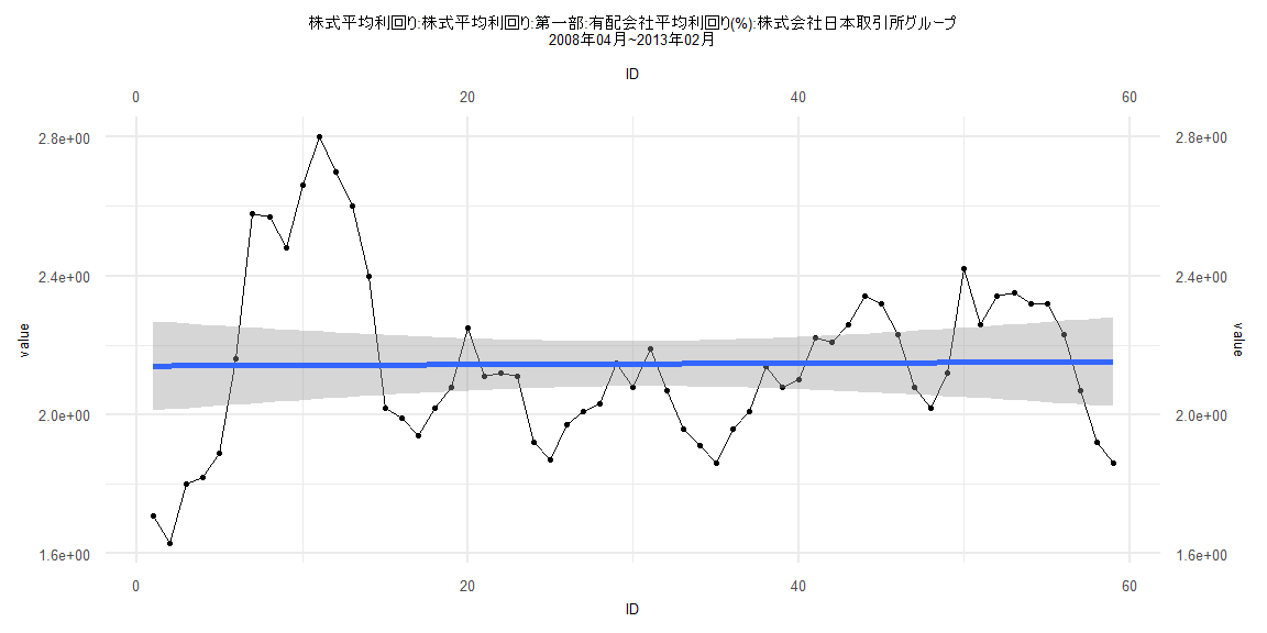
Call:
lm(formula = value ~ ID)

Residuals:
    Min      1Q  Median      3Q     Max
-0.5107 -0.1646 -0.0350  0.1397  0.6575

Coefficients:
             Estimate Std. Error t value            Pr(>|t|)
(Intercept) 2.1402864  0.0657170  32.568 <0.0000000000000002 ***
ID          0.0002051  0.0019050   0.108               0.915
---
Signif. codes:  0 '***' 0.001 '**' 0.01 '*' 0.05 '.' 0.1 ' ' 1

Residual standard error: 0.2492 on 57 degrees of freedom
Multiple R-squared:  0.0002034, Adjusted R-squared:  -0.01734
F-statistic: 0.0116 on 1 and 57 DF,  p-value: 0.9146


    Two-sample Kolmogorov-Smirnov test

data:  lm_residuals and rnorm(n = length(lm_residuals), mean = 0, sd = sd(lm_residuals))
D = 0.13559, p-value = 0.6544
alternative hypothesis: two-sided


    Durbin-Watson test

data:  value ~ ID
DW = 0.28655, p-value < 0.00000000000000022
alternative hypothesis: true autocorrelation is greater than 0


    studentized Breusch-Pagan test

data:  value ~ ID
BP = 15.441, df = 1, p-value = 0.0000851


    Box-Ljung test

data:  lm_residuals
X-squared = 41.568, df = 1, p-value = 0.0000000001139
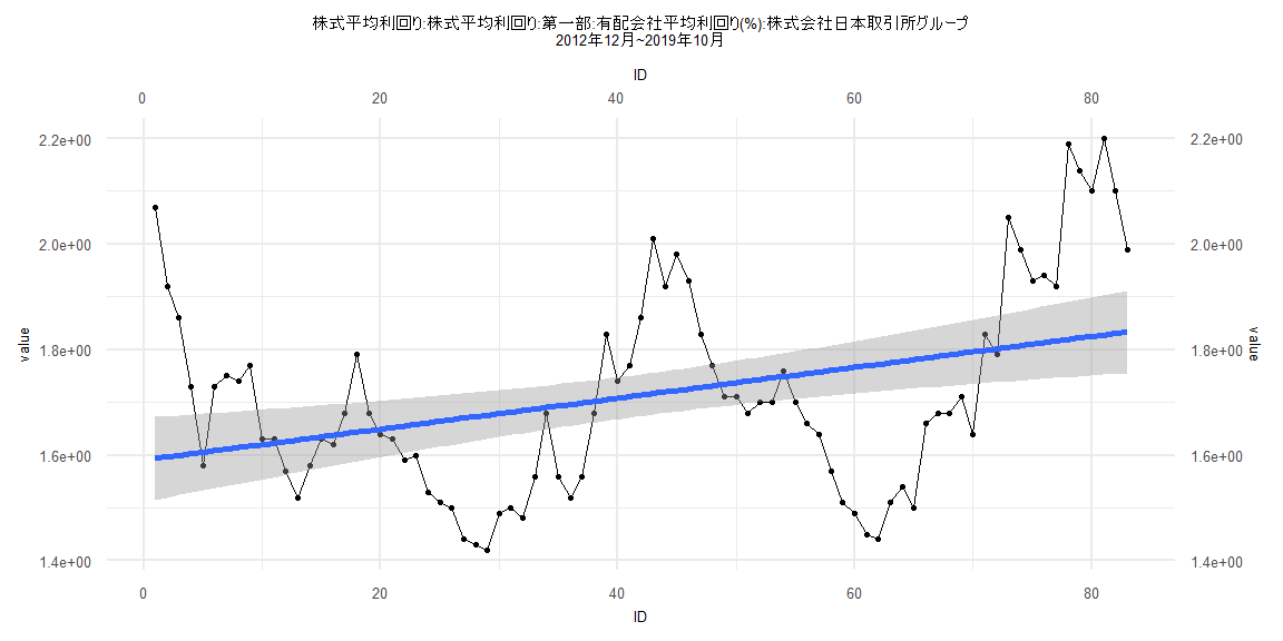
Call:
lm(formula = value ~ ID)

Residuals:
     Min       1Q   Median       3Q      Max
-0.33830 -0.11986 -0.00566  0.11547  0.34830

Coefficients:
             Estimate Std. Error t value             Pr(>|t|)
(Intercept) 1.5445285  0.0378691  40.786 < 0.0000000000000002 ***
ID          0.0039623  0.0008123   4.878           0.00000555 ***
---
Signif. codes:  0 '***' 0.001 '**' 0.01 '*' 0.05 '.' 0.1 ' ' 1

Residual standard error: 0.1678 on 78 degrees of freedom
Multiple R-squared:  0.2338,    Adjusted R-squared:  0.2239
F-statistic: 23.79 on 1 and 78 DF,  p-value: 0.00000555


    Two-sample Kolmogorov-Smirnov test

data:  lm_residuals and rnorm(n = length(lm_residuals), mean = 0, sd = sd(lm_residuals))
D = 0.1125, p-value = 0.6953
alternative hypothesis: two-sided


    Durbin-Watson test

data:  value ~ ID
DW = 0.25142, p-value < 0.00000000000000022
alternative hypothesis: true autocorrelation is greater than 0


    studentized Breusch-Pagan test

data:  value ~ ID
BP = 11.307, df = 1, p-value = 0.0007723


    Box-Ljung test

data:  lm_residuals
X-squared = 61.848, df = 1, p-value = 0.000000000000003664