Analysis
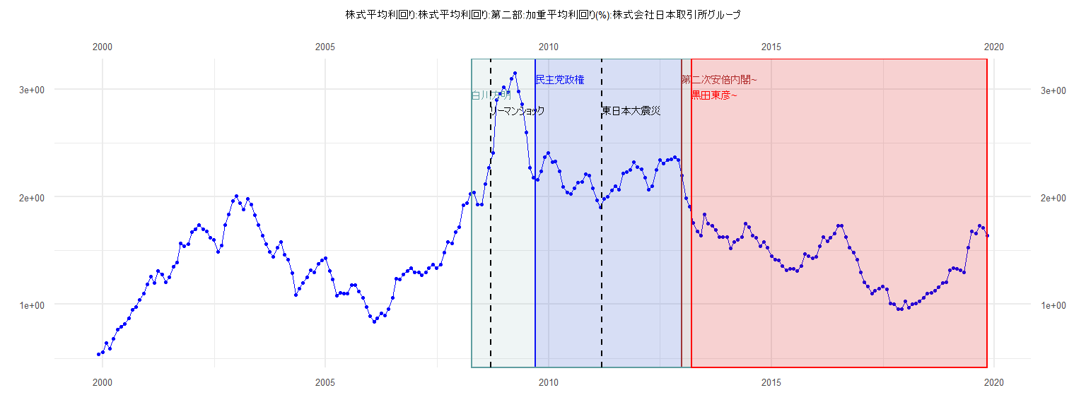
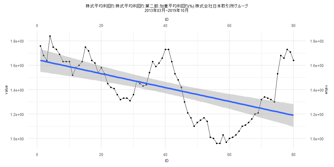
[1] "株式平均利回り:株式平均利回り:第二部:加重平均利回り(%):株式会社日本取引所グループ"
      Jan  Feb  Mar  Apr  May  Jun  Jul  Aug  Sep  Oct  Nov  Dec
1999                                                   0.54 0.56
2000 0.64 0.59 0.68 0.77 0.79 0.82 0.87 0.95 0.98 1.04 1.10 1.19
2001 1.26 1.20 1.31 1.28 1.21 1.25 1.35 1.39 1.57 1.54 1.56 1.67
2002 1.70 1.74 1.70 1.68 1.62 1.60 1.49 1.55 1.74 1.84 1.96 2.01
2003 1.94 1.88 1.98 1.93 1.83 1.74 1.64 1.56 1.49 1.44 1.53 1.58
2004 1.46 1.42 1.29 1.09 1.15 1.20 1.25 1.32 1.30 1.38 1.41 1.43
2005 1.31 1.23 1.08 1.11 1.10 1.10 1.18 1.18 1.12 1.06 0.98 0.89
2006 0.84 0.87 0.92 0.90 0.96 1.06 1.24 1.23 1.28 1.31 1.34 1.30
2007 1.30 1.27 1.30 1.34 1.37 1.34 1.37 1.48 1.58 1.57 1.67 1.72
2008 1.92 1.94 2.03 2.04 1.93 1.93 2.12 2.27 2.41 2.90 2.96 3.02
2009 2.97 3.10 3.15 2.98 2.86 2.60 2.27 2.18 2.16 2.24 2.37 2.41
2010 2.32 2.33 2.24 2.09 2.04 2.03 2.08 2.13 2.14 2.21 2.20 2.08
2011 1.97 1.90 1.98 2.00 2.06 2.10 2.07 2.22 2.23 2.25 2.32 2.28
2012 2.26 2.18 2.07 2.10 2.25 2.34 2.31 2.34 2.35 2.37 2.34 2.20
2013 1.99 1.91 1.76 1.68 1.64 1.84 1.75 1.73 1.69 1.63 1.63 1.63
2014 1.52 1.58 1.60 1.63 1.75 1.72 1.64 1.62 1.54 1.58 1.53 1.45
2015 1.42 1.41 1.36 1.32 1.33 1.33 1.31 1.36 1.47 1.45 1.43 1.44
2016 1.54 1.63 1.59 1.62 1.66 1.73 1.73 1.63 1.53 1.48 1.42 1.30
2017 1.21 1.17 1.10 1.13 1.15 1.17 1.14 1.01 1.00 0.96 0.96 1.03
2018 0.97 1.00 1.01 1.03 1.06 1.10 1.11 1.13 1.16 1.20 1.21 1.32
2019 1.34 1.33 1.32 1.30 1.53 1.68 1.66 1.73 1.71 1.64
Call:
lm(formula = value ~ ID)

Residuals:
     Min       1Q   Median       3Q      Max
-0.28379 -0.10858  0.02361  0.10005  0.26073

Coefficients:
            Estimate Std. Error t value            Pr(>|t|)
(Intercept) 2.139406   0.042816  49.968 <0.0000000000000002 ***
ID          0.002466   0.001866   1.322               0.194
---
Signif. codes:  0 '***' 0.001 '**' 0.01 '*' 0.05 '.' 0.1 ' ' 1

Residual standard error: 0.1311 on 37 degrees of freedom
Multiple R-squared:  0.04508,   Adjusted R-squared:  0.01927
F-statistic: 1.747 on 1 and 37 DF,  p-value: 0.1944


    Two-sample Kolmogorov-Smirnov test

data:  lm_residuals and rnorm(n = length(lm_residuals), mean = 0, sd = sd(lm_residuals))
D = 0.17949, p-value = 0.5622
alternative hypothesis: two-sided


    Durbin-Watson test

data:  value ~ ID
DW = 0.3193, p-value = 0.0000000000002655
alternative hypothesis: true autocorrelation is greater than 0


    studentized Breusch-Pagan test

data:  value ~ ID
BP = 2.2632, df = 1, p-value = 0.1325


    Box-Ljung test

data:  lm_residuals
X-squared = 29.094, df = 1, p-value = 0.00000006894
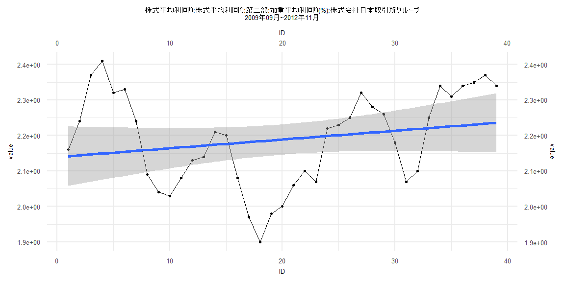
Call:
lm(formula = value ~ ID)

Residuals:
     Min       1Q   Median       3Q      Max
-0.36385 -0.17238 -0.02076  0.11463  0.55302

Coefficients:
             Estimate Std. Error t value             Pr(>|t|)
(Intercept)  1.717752   0.048667  35.296 < 0.0000000000000002 ***
ID          -0.006676   0.001006  -6.633        0.00000000341 ***
---
Signif. codes:  0 '***' 0.001 '**' 0.01 '*' 0.05 '.' 0.1 ' ' 1

Residual standard error: 0.2197 on 81 degrees of freedom
Multiple R-squared:  0.352, Adjusted R-squared:  0.344
F-statistic:    44 on 1 and 81 DF,  p-value: 0.000000003411


    Two-sample Kolmogorov-Smirnov test

data:  lm_residuals and rnorm(n = length(lm_residuals), mean = 0, sd = sd(lm_residuals))
D = 0.084337, p-value = 0.9317
alternative hypothesis: two-sided


    Durbin-Watson test

data:  value ~ ID
DW = 0.10897, p-value < 0.00000000000000022
alternative hypothesis: true autocorrelation is greater than 0


    studentized Breusch-Pagan test

data:  value ~ ID
BP = 15.964, df = 1, p-value = 0.00006456


    Box-Ljung test

data:  lm_residuals
X-squared = 67.526, df = 1, p-value = 0.000000000000000222
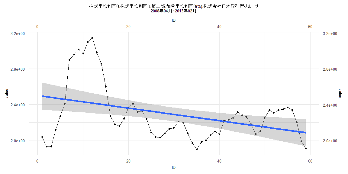
Call:
lm(formula = value ~ ID)

Residuals:
     Min       1Q   Median       3Q      Max
-0.55802 -0.19321 -0.05677  0.15118  0.73246

Coefficients:
             Estimate Std. Error t value             Pr(>|t|)
(Intercept)  2.502116   0.077684   32.21 < 0.0000000000000002 ***
ID          -0.007048   0.002252   -3.13              0.00276 **
---
Signif. codes:  0 '***' 0.001 '**' 0.01 '*' 0.05 '.' 0.1 ' ' 1

Residual standard error: 0.2946 on 57 degrees of freedom
Multiple R-squared:  0.1466,    Adjusted R-squared:  0.1317
F-statistic: 9.795 on 1 and 57 DF,  p-value: 0.002758


    Two-sample Kolmogorov-Smirnov test

data:  lm_residuals and rnorm(n = length(lm_residuals), mean = 0, sd = sd(lm_residuals))
D = 0.10169, p-value = 0.9239
alternative hypothesis: two-sided


    Durbin-Watson test

data:  value ~ ID
DW = 0.17444, p-value < 0.00000000000000022
alternative hypothesis: true autocorrelation is greater than 0


    studentized Breusch-Pagan test

data:  value ~ ID
BP = 19.041, df = 1, p-value = 0.0000128


    Box-Ljung test

data:  lm_residuals
X-squared = 49.008, df = 1, p-value = 0.000000000002549
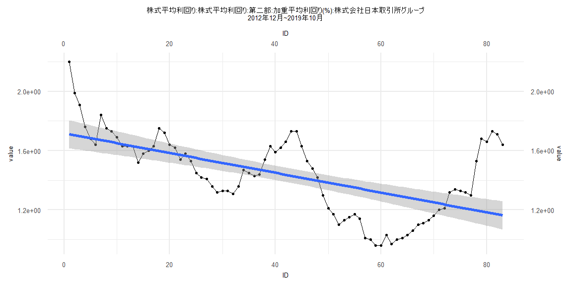
Call:
lm(formula = value ~ ID)

Residuals:
     Min       1Q   Median       3Q      Max
-0.36650 -0.16580  0.00296  0.10386  0.52912

Coefficients:
             Estimate Std. Error t value             Pr(>|t|)
(Intercept)  1.646247   0.047757  34.471 < 0.0000000000000002 ***
ID          -0.005710   0.001024  -5.574          0.000000343 ***
---
Signif. codes:  0 '***' 0.001 '**' 0.01 '*' 0.05 '.' 0.1 ' ' 1

Residual standard error: 0.2116 on 78 degrees of freedom
Multiple R-squared:  0.2849,    Adjusted R-squared:  0.2757
F-statistic: 31.07 on 1 and 78 DF,  p-value: 0.0000003434


    Two-sample Kolmogorov-Smirnov test

data:  lm_residuals and rnorm(n = length(lm_residuals), mean = 0, sd = sd(lm_residuals))
D = 0.2, p-value = 0.08141
alternative hypothesis: two-sided


    Durbin-Watson test

data:  value ~ ID
DW = 0.10253, p-value < 0.00000000000000022
alternative hypothesis: true autocorrelation is greater than 0


    studentized Breusch-Pagan test

data:  value ~ ID
BP = 24.667, df = 1, p-value = 0.0000006816


    Box-Ljung test

data:  lm_residuals
X-squared = 69.921, df = 1, p-value < 0.00000000000000022