Analysis
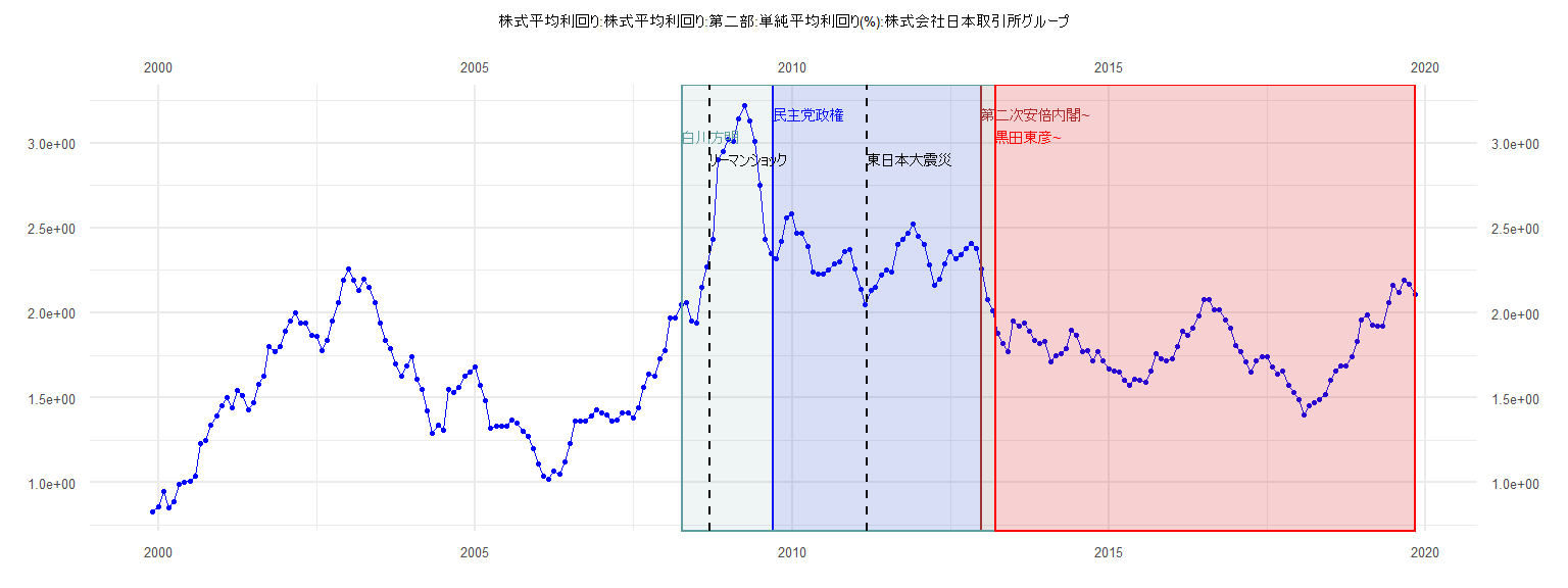
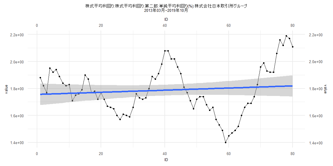
[1] "株式平均利回り:株式平均利回り:第二部:単純平均利回り(%):株式会社日本取引所グループ"
      Jan  Feb  Mar  Apr  May  Jun  Jul  Aug  Sep  Oct  Nov  Dec
1999                                                   0.83 0.86
2000 0.95 0.85 0.89 0.99 1.00 1.01 1.04 1.23 1.25 1.34 1.39 1.45
2001 1.50 1.44 1.54 1.51 1.43 1.47 1.58 1.63 1.80 1.77 1.80 1.89
2002 1.95 2.00 1.94 1.94 1.87 1.86 1.78 1.84 1.95 2.06 2.19 2.26
2003 2.19 2.13 2.20 2.15 2.06 1.94 1.84 1.79 1.70 1.63 1.69 1.74
2004 1.61 1.55 1.42 1.29 1.34 1.31 1.55 1.53 1.56 1.63 1.65 1.68
2005 1.57 1.48 1.32 1.33 1.33 1.33 1.37 1.35 1.30 1.27 1.20 1.11
2006 1.04 1.02 1.07 1.05 1.12 1.23 1.36 1.36 1.36 1.39 1.43 1.41
2007 1.40 1.36 1.37 1.41 1.41 1.38 1.44 1.56 1.64 1.63 1.73 1.78
2008 1.97 1.97 2.05 2.06 1.95 1.94 2.15 2.27 2.43 2.90 2.95 3.02
2009 3.01 3.14 3.22 3.13 3.01 2.75 2.43 2.35 2.32 2.42 2.56 2.58
2010 2.47 2.47 2.39 2.24 2.23 2.23 2.25 2.29 2.30 2.36 2.37 2.26
2011 2.14 2.05 2.13 2.15 2.22 2.25 2.24 2.40 2.43 2.47 2.52 2.45
2012 2.40 2.28 2.16 2.20 2.29 2.36 2.32 2.34 2.38 2.41 2.38 2.26
2013 2.08 2.01 1.88 1.82 1.77 1.95 1.92 1.94 1.89 1.84 1.82 1.83
2014 1.71 1.75 1.76 1.79 1.90 1.87 1.77 1.78 1.72 1.77 1.72 1.67
2015 1.66 1.65 1.60 1.57 1.61 1.60 1.59 1.66 1.76 1.73 1.72 1.73
2016 1.80 1.89 1.87 1.91 1.98 2.08 2.08 2.02 2.02 1.96 1.91 1.81
2017 1.77 1.71 1.65 1.72 1.74 1.74 1.68 1.64 1.66 1.57 1.53 1.49
2018 1.40 1.45 1.47 1.49 1.52 1.60 1.66 1.69 1.69 1.74 1.83 1.96
2019 1.99 1.93 1.92 1.92 2.06 2.16 2.12 2.19 2.17 2.11
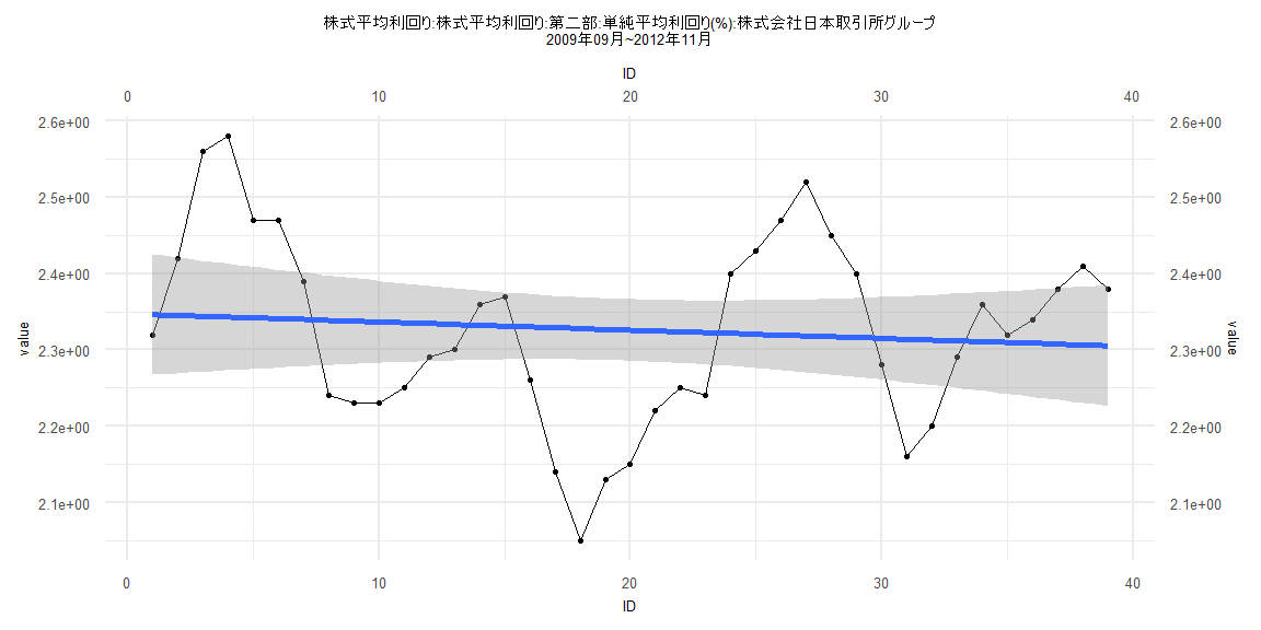
Call:
lm(formula = value ~ ID)

Residuals:
     Min       1Q   Median       3Q      Max
-0.27804 -0.09216  0.01020  0.08108  0.23694

Coefficients:
             Estimate Std. Error t value            Pr(>|t|)
(Intercept)  2.347355   0.040536  57.908 <0.0000000000000002 ***
ID          -0.001073   0.001766  -0.607               0.547
---
Signif. codes:  0 '***' 0.001 '**' 0.01 '*' 0.05 '.' 0.1 ' ' 1

Residual standard error: 0.1241 on 37 degrees of freedom
Multiple R-squared:  0.009873,  Adjusted R-squared:  -0.01689
F-statistic: 0.3689 on 1 and 37 DF,  p-value: 0.5473


    Two-sample Kolmogorov-Smirnov test

data:  lm_residuals and rnorm(n = length(lm_residuals), mean = 0, sd = sd(lm_residuals))
D = 0.12821, p-value = 0.9114
alternative hypothesis: two-sided


    Durbin-Watson test

data:  value ~ ID
DW = 0.37031, p-value = 0.000000000004823
alternative hypothesis: true autocorrelation is greater than 0


    studentized Breusch-Pagan test

data:  value ~ ID
BP = 1.4859, df = 1, p-value = 0.2229


    Box-Ljung test

data:  lm_residuals
X-squared = 27.565, df = 1, p-value = 0.0000001519
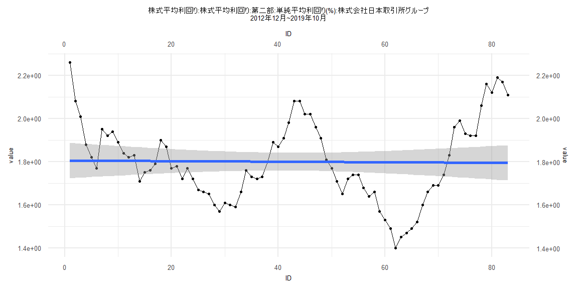
Call:
lm(formula = value ~ ID)

Residuals:
    Min      1Q  Median      3Q     Max
-0.3975 -0.1344 -0.0324  0.1244  0.4548

Coefficients:
              Estimate Std. Error t value            Pr(>|t|)
(Intercept)  1.8053071  0.0417864  43.203 <0.0000000000000002 ***
ID          -0.0001264  0.0008642  -0.146               0.884
---
Signif. codes:  0 '***' 0.001 '**' 0.01 '*' 0.05 '.' 0.1 ' ' 1

Residual standard error: 0.1886 on 81 degrees of freedom
Multiple R-squared:  0.0002639, Adjusted R-squared:  -0.01208
F-statistic: 0.02138 on 1 and 81 DF,  p-value: 0.8841


    Two-sample Kolmogorov-Smirnov test

data:  lm_residuals and rnorm(n = length(lm_residuals), mean = 0, sd = sd(lm_residuals))
D = 0.072289, p-value = 0.9829
alternative hypothesis: two-sided


    Durbin-Watson test

data:  value ~ ID
DW = 0.12077, p-value < 0.00000000000000022
alternative hypothesis: true autocorrelation is greater than 0


    studentized Breusch-Pagan test

data:  value ~ ID
BP = 10.41, df = 1, p-value = 0.001253


    Box-Ljung test

data:  lm_residuals
X-squared = 67.614, df = 1, p-value = 0.000000000000000222
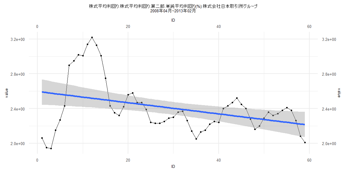
Call:
lm(formula = value ~ ID)

Residuals:
     Min       1Q   Median       3Q      Max
-0.63725 -0.15122 -0.03642  0.12556  0.70087

Coefficients:
             Estimate Std. Error t value            Pr(>|t|)
(Intercept)  2.596628   0.074264   34.97 <0.0000000000000002 ***
ID          -0.006458   0.002153   -3.00               0.004 **
---
Signif. codes:  0 '***' 0.001 '**' 0.01 '*' 0.05 '.' 0.1 ' ' 1

Residual standard error: 0.2816 on 57 degrees of freedom
Multiple R-squared:  0.1364,    Adjusted R-squared:  0.1212
F-statistic: 8.999 on 1 and 57 DF,  p-value: 0.004


    Two-sample Kolmogorov-Smirnov test

data:  lm_residuals and rnorm(n = length(lm_residuals), mean = 0, sd = sd(lm_residuals))
D = 0.22034, p-value = 0.1141
alternative hypothesis: two-sided


    Durbin-Watson test

data:  value ~ ID
DW = 0.17971, p-value < 0.00000000000000022
alternative hypothesis: true autocorrelation is greater than 0


    studentized Breusch-Pagan test

data:  value ~ ID
BP = 21.918, df = 1, p-value = 0.000002845


    Box-Ljung test

data:  lm_residuals
X-squared = 47.441, df = 1, p-value = 0.000000000005669
Call:
lm(formula = value ~ ID)

Residuals:
     Min       1Q   Median       3Q      Max
-0.40272 -0.11923 -0.00419  0.12324  0.37229

Coefficients:
             Estimate Std. Error t value            Pr(>|t|)
(Intercept) 1.7561741  0.0404980  43.364 <0.0000000000000002 ***
ID          0.0007889  0.0008687   0.908               0.367
---
Signif. codes:  0 '***' 0.001 '**' 0.01 '*' 0.05 '.' 0.1 ' ' 1

Residual standard error: 0.1794 on 78 degrees of freedom
Multiple R-squared:  0.01046,   Adjusted R-squared:  -0.002223
F-statistic: 0.8248 on 1 and 78 DF,  p-value: 0.3666


    Two-sample Kolmogorov-Smirnov test

data:  lm_residuals and rnorm(n = length(lm_residuals), mean = 0, sd = sd(lm_residuals))
D = 0.1375, p-value = 0.4383
alternative hypothesis: two-sided


    Durbin-Watson test

data:  value ~ ID
DW = 0.11693, p-value < 0.00000000000000022
alternative hypothesis: true autocorrelation is greater than 0


    studentized Breusch-Pagan test

data:  value ~ ID
BP = 20.377, df = 1, p-value = 0.000006359


    Box-Ljung test

data:  lm_residuals
X-squared = 70.542, df = 1, p-value < 0.00000000000000022