Analysis
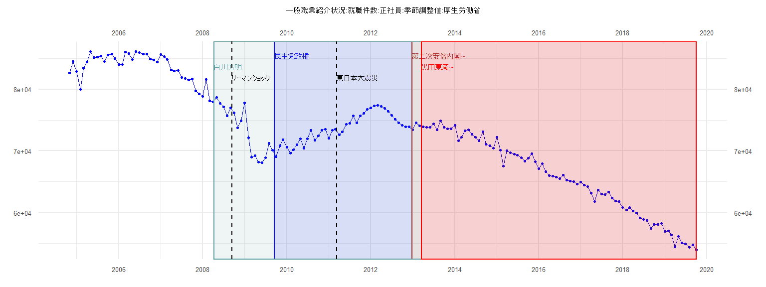
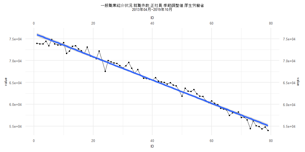
[1] "一般職業紹介状況:就職件数:正社員:季節調整値:厚生労働省"
       Jan   Feb   Mar   Apr   May   Jun   Jul   Aug   Sep   Oct   Nov   Dec
2004                                                             82614 84440
2005 82866 79991 83400 84426 86089 85121 85194 85353 84487 85550 85710 84968
2006 83966 83986 85990 85794 84806 86080 85924 85703 85712 84876 84750 84395
2007 85615 85247 84841 83116 82951 83000 81867 81715 81489 81668 79704 79222
2008 78818 81574 78070 77909 78695 77707 77110 75661 77013 76158 73723 74904
2009 77800 72131 69015 69199 68222 68122 68886 71276 70104 69045 70815 71823
2010 70609 69666 70214 71042 71965 70404 71940 73325 71760 72482 73373 73482
2011 72069 73350 73527 72618 73067 74277 74492 75668 74590 75678 76124 76765
2012 76991 77268 77370 77250 76925 76415 75804 75158 74576 74171 73950 73899
2013 73433 74589 74043 73937 73852 73850 74423 73425 74888 73817 73608 73612
2014 74165 71673 72183 73277 73439 72694 72244 71656 73101 71074 70831 70423
2015 72192 70126 67550 70025 69736 69498 69340 68910 68308 68796 69579 68251
2016 67106 67965 66669 66011 65905 65760 65557 66075 65318 65124 65027 64623
2017 64964 64439 64229 63196 61846 63655 63000 62977 63360 62404 61852 61817
2018 60822 60443 60804 60270 59939 59110 58914 58711 57486 58090 58075 58267
2019 56965 57053 56430 54462 56178 55105 54916 54383 54792 54020
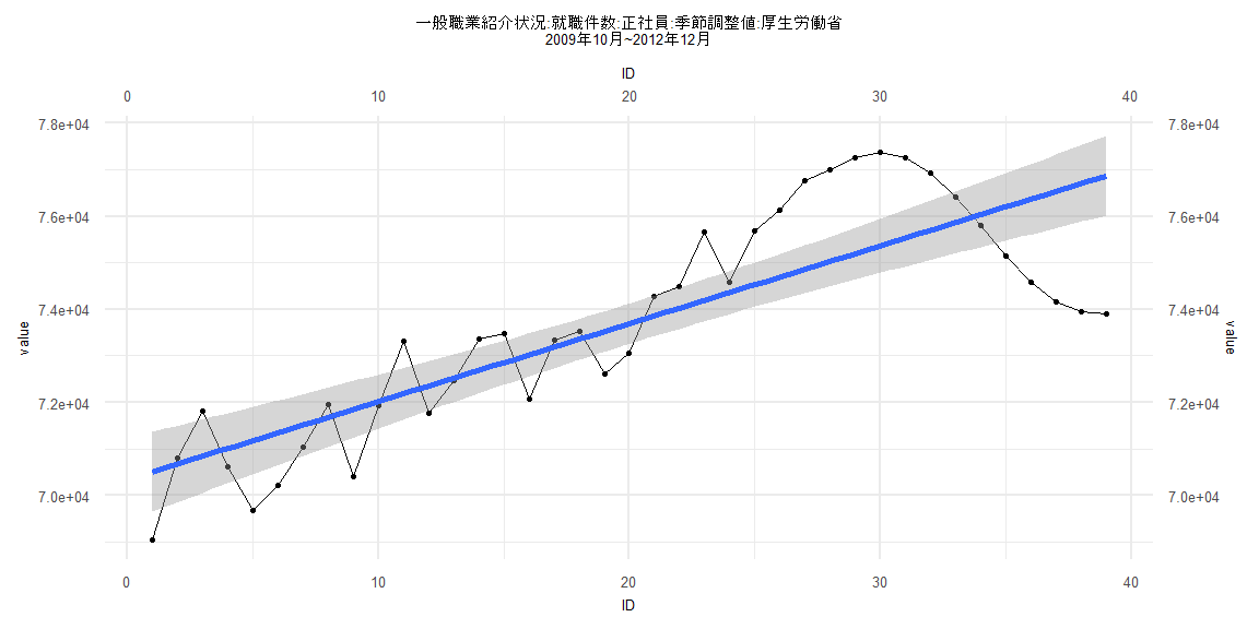
Call:
lm(formula = value ~ ID)

Residuals:
    Min      1Q  Median      3Q     Max
-2973.1  -928.9   161.3  1059.6  2070.2

Coefficients:
            Estimate Std. Error t value             Pr(>|t|)
(Intercept) 70342.41     438.84 160.293 < 0.0000000000000002 ***
ID            167.43      19.12   8.756       0.000000000151 ***
---
Signif. codes:  0 '***' 0.001 '**' 0.01 '*' 0.05 '.' 0.1 ' ' 1

Residual standard error: 1344 on 37 degrees of freedom
Multiple R-squared:  0.6745,    Adjusted R-squared:  0.6657
F-statistic: 76.66 on 1 and 37 DF,  p-value: 0.0000000001507


    Two-sample Kolmogorov-Smirnov test

data:  lm_residuals and rnorm(n = length(lm_residuals), mean = 0, sd = sd(lm_residuals))
D = 0.15385, p-value = 0.7523
alternative hypothesis: two-sided


    Durbin-Watson test

data:  value ~ ID
DW = 0.45918, p-value = 0.0000000002909
alternative hypothesis: true autocorrelation is greater than 0


    studentized Breusch-Pagan test

data:  value ~ ID
BP = 12.665, df = 1, p-value = 0.0003726


    Box-Ljung test

data:  lm_residuals
X-squared = 19.931, df = 1, p-value = 0.000008028
Call:
lm(formula = value ~ ID)

Residuals:
    Min      1Q  Median      3Q     Max
-2988.7  -432.5   136.7   654.5  2028.1

Coefficients:
             Estimate Std. Error t value            Pr(>|t|)
(Intercept) 76682.395    221.964  345.47 <0.0000000000000002 ***
ID           -260.739      4.646  -56.12 <0.0000000000000002 ***
---
Signif. codes:  0 '***' 0.001 '**' 0.01 '*' 0.05 '.' 0.1 ' ' 1

Residual standard error: 995.8 on 80 degrees of freedom
Multiple R-squared:  0.9752,    Adjusted R-squared:  0.9749
F-statistic:  3150 on 1 and 80 DF,  p-value: < 0.00000000000000022


    Two-sample Kolmogorov-Smirnov test

data:  lm_residuals and rnorm(n = length(lm_residuals), mean = 0, sd = sd(lm_residuals))
D = 0.10976, p-value = 0.7099
alternative hypothesis: two-sided


    Durbin-Watson test

data:  value ~ ID
DW = 0.88055, p-value = 0.000000006249
alternative hypothesis: true autocorrelation is greater than 0


    studentized Breusch-Pagan test

data:  value ~ ID
BP = 3.8296, df = 1, p-value = 0.05036


    Box-Ljung test

data:  lm_residuals
X-squared = 20.674, df = 1, p-value = 0.000005444
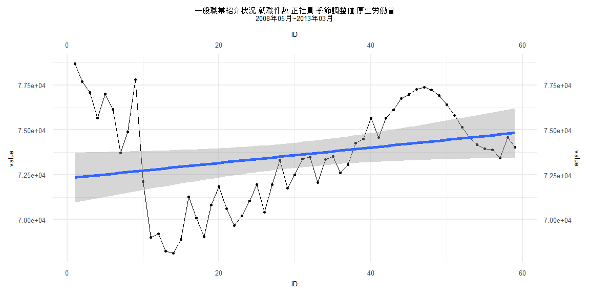
Call:
lm(formula = value ~ ID)

Residuals:
    Min      1Q  Median      3Q     Max
-4780.5 -1680.4  -276.2  1973.0  6350.1

Coefficients:
            Estimate Std. Error t value            Pr(>|t|)
(Intercept) 72302.01     710.41 101.775 <0.0000000000000002 ***
ID             42.89      20.59   2.083              0.0418 *
---
Signif. codes:  0 '***' 0.001 '**' 0.01 '*' 0.05 '.' 0.1 ' ' 1

Residual standard error: 2694 on 57 degrees of freedom
Multiple R-squared:  0.07072,   Adjusted R-squared:  0.05442
F-statistic: 4.338 on 1 and 57 DF,  p-value: 0.04177


    Two-sample Kolmogorov-Smirnov test

data:  lm_residuals and rnorm(n = length(lm_residuals), mean = 0, sd = sd(lm_residuals))
D = 0.15254, p-value = 0.5021
alternative hypothesis: two-sided


    Durbin-Watson test

data:  value ~ ID
DW = 0.25856, p-value < 0.00000000000000022
alternative hypothesis: true autocorrelation is greater than 0


    studentized Breusch-Pagan test

data:  value ~ ID
BP = 23.663, df = 1, p-value = 0.000001148


    Box-Ljung test

data:  lm_residuals
X-squared = 41.848, df = 1, p-value = 0.00000000009865
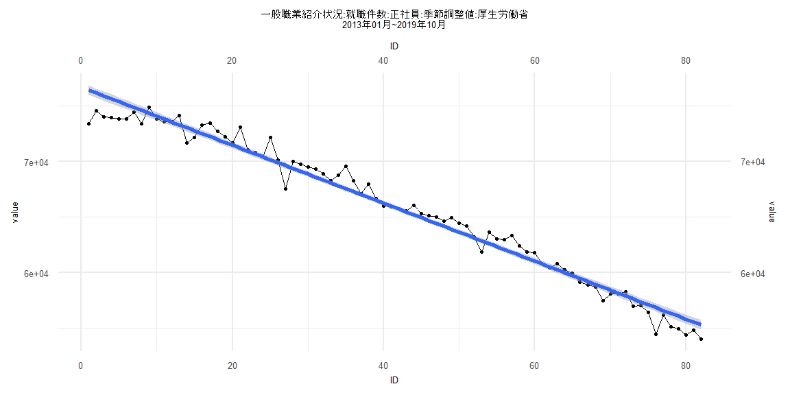
Call:
lm(formula = value ~ ID)

Residuals:
     Min       1Q   Median       3Q      Max
-2276.61  -417.86    48.45   578.48  1889.77

Coefficients:
             Estimate Std. Error t value            Pr(>|t|)
(Intercept) 76238.727    204.269  373.23 <0.0000000000000002 ***
ID           -267.172      4.436  -60.22 <0.0000000000000002 ***
---
Signif. codes:  0 '***' 0.001 '**' 0.01 '*' 0.05 '.' 0.1 ' ' 1

Residual standard error: 899.2 on 77 degrees of freedom
Multiple R-squared:  0.9792,    Adjusted R-squared:  0.9789
F-statistic:  3627 on 1 and 77 DF,  p-value: < 0.00000000000000022


    Two-sample Kolmogorov-Smirnov test

data:  lm_residuals and rnorm(n = length(lm_residuals), mean = 0, sd = sd(lm_residuals))
D = 0.12658, p-value = 0.5543
alternative hypothesis: two-sided


    Durbin-Watson test

data:  value ~ ID
DW = 1.0882, p-value = 0.000004773
alternative hypothesis: true autocorrelation is greater than 0


    studentized Breusch-Pagan test

data:  value ~ ID
BP = 2.0811, df = 1, p-value = 0.1491


    Box-Ljung test

data:  lm_residuals
X-squared = 13.973, df = 1, p-value = 0.0001854