Analysis
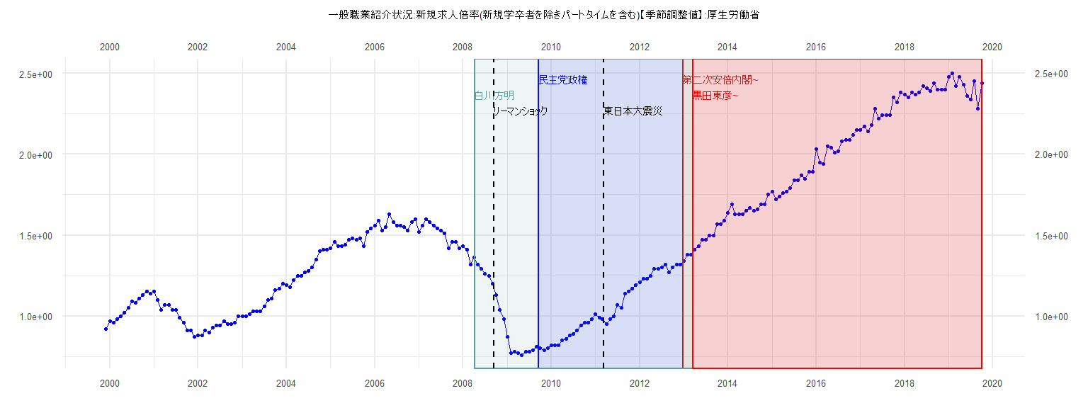
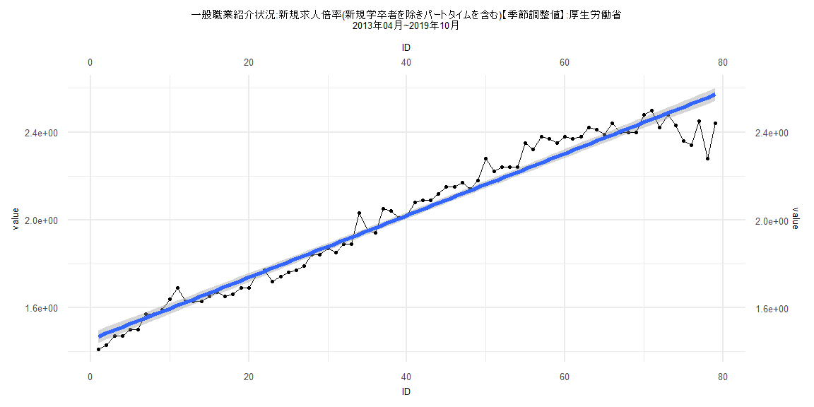
[1] "一般職業紹介状況:新規求人倍率(新規学卒者を除きパートタイムを含む)【季節調整値】:厚生労働省"
      Jan  Feb  Mar  Apr  May  Jun  Jul  Aug  Sep  Oct  Nov  Dec
1999                                                        0.92
2000 0.97 0.96 0.98 1.00 1.02 1.05 1.09 1.08 1.11 1.13 1.15 1.14
2001 1.15 1.10 1.04 1.07 1.07 1.04 1.04 0.99 0.96 0.91 0.91 0.87
2002 0.88 0.88 0.91 0.90 0.93 0.94 0.94 0.97 0.95 0.95 0.96 1.00
2003 1.00 1.00 1.01 1.03 1.03 1.03 1.06 1.10 1.11 1.16 1.17 1.20
2004 1.19 1.18 1.22 1.25 1.25 1.27 1.28 1.30 1.35 1.40 1.41 1.41
2005 1.42 1.46 1.43 1.43 1.44 1.47 1.48 1.47 1.48 1.43 1.52 1.54
2006 1.56 1.59 1.53 1.55 1.63 1.58 1.56 1.56 1.55 1.53 1.58 1.60
2007 1.52 1.56 1.60 1.58 1.56 1.54 1.53 1.51 1.42 1.46 1.46 1.42
2008 1.43 1.41 1.32 1.36 1.32 1.29 1.26 1.25 1.20 1.13 1.04 0.98
2009 0.87 0.77 0.78 0.77 0.76 0.78 0.78 0.79 0.81 0.80 0.79 0.80
2010 0.82 0.82 0.82 0.85 0.86 0.88 0.89 0.91 0.94 0.96 0.96 0.98
2011 1.01 0.99 0.98 0.95 0.98 1.00 1.07 1.05 1.14 1.15 1.17 1.19
2012 1.21 1.23 1.23 1.25 1.29 1.29 1.30 1.32 1.27 1.30 1.32 1.32
2013 1.34 1.38 1.38 1.41 1.43 1.47 1.47 1.50 1.50 1.57 1.57 1.59
2014 1.64 1.69 1.63 1.63 1.63 1.65 1.67 1.65 1.66 1.69 1.69 1.75
2015 1.77 1.72 1.74 1.76 1.77 1.79 1.84 1.84 1.87 1.85 1.89 1.89
2016 2.03 1.95 1.94 2.05 2.04 2.01 2.02 2.08 2.09 2.09 2.12 2.15
2017 2.15 2.17 2.14 2.18 2.28 2.22 2.24 2.24 2.24 2.35 2.32 2.38
2018 2.37 2.35 2.38 2.37 2.38 2.42 2.41 2.39 2.44 2.40 2.40 2.40
2019 2.48 2.50 2.42 2.48 2.43 2.36 2.34 2.45 2.28 2.44
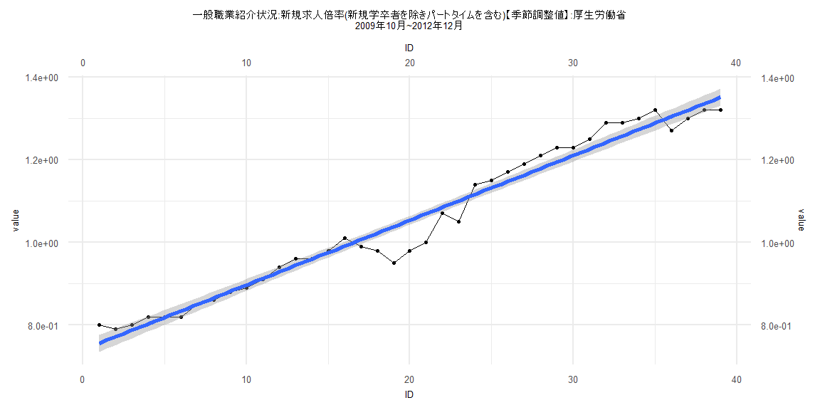
Call:
lm(formula = value ~ ID)

Residuals:
     Min       1Q   Median       3Q      Max
-0.08793 -0.01523  0.00473  0.02309  0.04844

Coefficients:
             Estimate Std. Error t value            Pr(>|t|)
(Intercept) 0.7403104  0.0107115   69.11 <0.0000000000000002 ***
ID          0.0156640  0.0004667   33.56 <0.0000000000000002 ***
---
Signif. codes:  0 '***' 0.001 '**' 0.01 '*' 0.05 '.' 0.1 ' ' 1

Residual standard error: 0.03281 on 37 degrees of freedom
Multiple R-squared:  0.9682,    Adjusted R-squared:  0.9673
F-statistic:  1126 on 1 and 37 DF,  p-value: < 0.00000000000000022


    Two-sample Kolmogorov-Smirnov test

data:  lm_residuals and rnorm(n = length(lm_residuals), mean = 0, sd = sd(lm_residuals))
D = 0.25641, p-value = 0.1547
alternative hypothesis: two-sided


    Durbin-Watson test

data:  value ~ ID
DW = 0.55835, p-value = 0.00000001066
alternative hypothesis: true autocorrelation is greater than 0


    studentized Breusch-Pagan test

data:  value ~ ID
BP = 0.77062, df = 1, p-value = 0.38


    Box-Ljung test

data:  lm_residuals
X-squared = 19.702, df = 1, p-value = 0.000009051
Call:
lm(formula = value ~ ID)

Residuals:
      Min        1Q    Median        3Q       Max
-0.282399 -0.036883  0.003114  0.046774  0.118944

Coefficients:
             Estimate Std. Error t value            Pr(>|t|)
(Intercept) 1.4013731  0.0148836   94.16 <0.0000000000000002 ***
ID          0.0143336  0.0003115   46.01 <0.0000000000000002 ***
---
Signif. codes:  0 '***' 0.001 '**' 0.01 '*' 0.05 '.' 0.1 ' ' 1

Residual standard error: 0.06677 on 80 degrees of freedom
Multiple R-squared:  0.9636,    Adjusted R-squared:  0.9631
F-statistic:  2117 on 1 and 80 DF,  p-value: < 0.00000000000000022


    Two-sample Kolmogorov-Smirnov test

data:  lm_residuals and rnorm(n = length(lm_residuals), mean = 0, sd = sd(lm_residuals))
D = 0.12195, p-value = 0.5785
alternative hypothesis: two-sided


    Durbin-Watson test

data:  value ~ ID
DW = 0.5526, p-value = 0.0000000000000008823
alternative hypothesis: true autocorrelation is greater than 0


    studentized Breusch-Pagan test

data:  value ~ ID
BP = 11.229, df = 1, p-value = 0.0008052


    Box-Ljung test

data:  lm_residuals
X-squared = 40.423, df = 1, p-value = 0.0000000002046
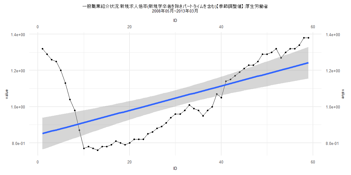
Call:
lm(formula = value ~ ID)

Residuals:
     Min       1Q   Median       3Q      Max
-0.18283 -0.14109 -0.05716  0.10123  0.46846

Coefficients:
            Estimate Std. Error t value             Pr(>|t|)
(Intercept) 0.844804   0.044769  18.870 < 0.0000000000000002 ***
ID          0.006738   0.001298   5.192           0.00000289 ***
---
Signif. codes:  0 '***' 0.001 '**' 0.01 '*' 0.05 '.' 0.1 ' ' 1

Residual standard error: 0.1698 on 57 degrees of freedom
Multiple R-squared:  0.3211,    Adjusted R-squared:  0.3092
F-statistic: 26.96 on 1 and 57 DF,  p-value: 0.000002892


    Two-sample Kolmogorov-Smirnov test

data:  lm_residuals and rnorm(n = length(lm_residuals), mean = 0, sd = sd(lm_residuals))
D = 0.22034, p-value = 0.1141
alternative hypothesis: two-sided


    Durbin-Watson test

data:  value ~ ID
DW = 0.047135, p-value < 0.00000000000000022
alternative hypothesis: true autocorrelation is greater than 0


    studentized Breusch-Pagan test

data:  value ~ ID
BP = 19.669, df = 1, p-value = 0.00000921


    Box-Ljung test

data:  lm_residuals
X-squared = 50.695, df = 1, p-value = 0.000000000001079
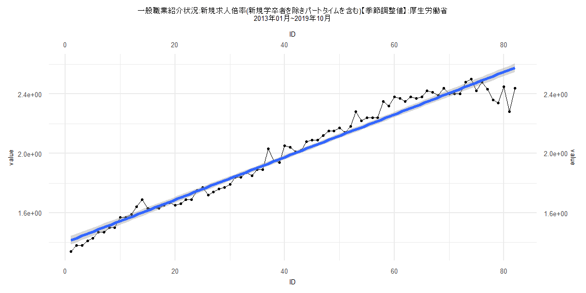
Call:
lm(formula = value ~ ID)

Residuals:
      Min        1Q    Median        3Q       Max
-0.277584 -0.036177  0.000592  0.045371  0.119432

Coefficients:
            Estimate Std. Error t value            Pr(>|t|)
(Intercept) 1.454382   0.015148   96.01 <0.0000000000000002 ***
ID          0.014144   0.000329   42.99 <0.0000000000000002 ***
---
Signif. codes:  0 '***' 0.001 '**' 0.01 '*' 0.05 '.' 0.1 ' ' 1

Residual standard error: 0.06668 on 77 degrees of freedom
Multiple R-squared:   0.96, Adjusted R-squared:  0.9595
F-statistic:  1848 on 1 and 77 DF,  p-value: < 0.00000000000000022


    Two-sample Kolmogorov-Smirnov test

data:  lm_residuals and rnorm(n = length(lm_residuals), mean = 0, sd = sd(lm_residuals))
D = 0.11392, p-value = 0.6878
alternative hypothesis: two-sided


    Durbin-Watson test

data:  value ~ ID
DW = 0.57238, p-value = 0.000000000000009171
alternative hypothesis: true autocorrelation is greater than 0


    studentized Breusch-Pagan test

data:  value ~ ID
BP = 11.471, df = 1, p-value = 0.0007069


    Box-Ljung test

data:  lm_residuals
X-squared = 38.322, df = 1, p-value = 0.0000000005998