Analysis
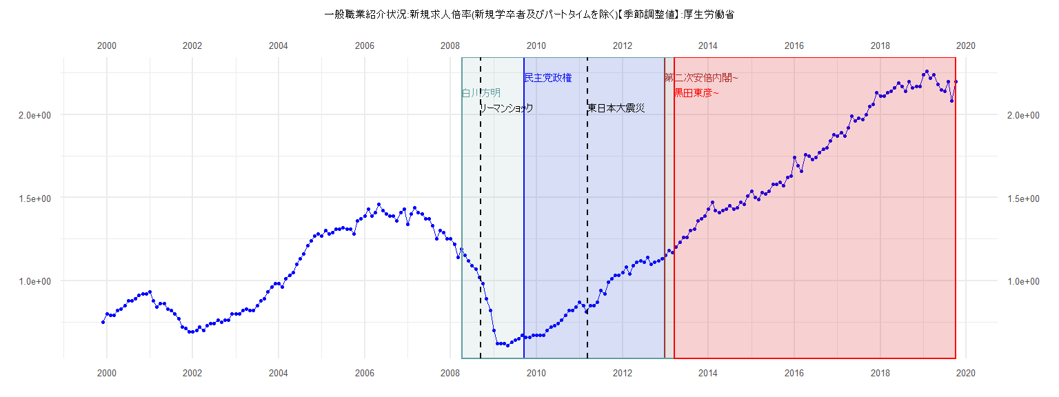
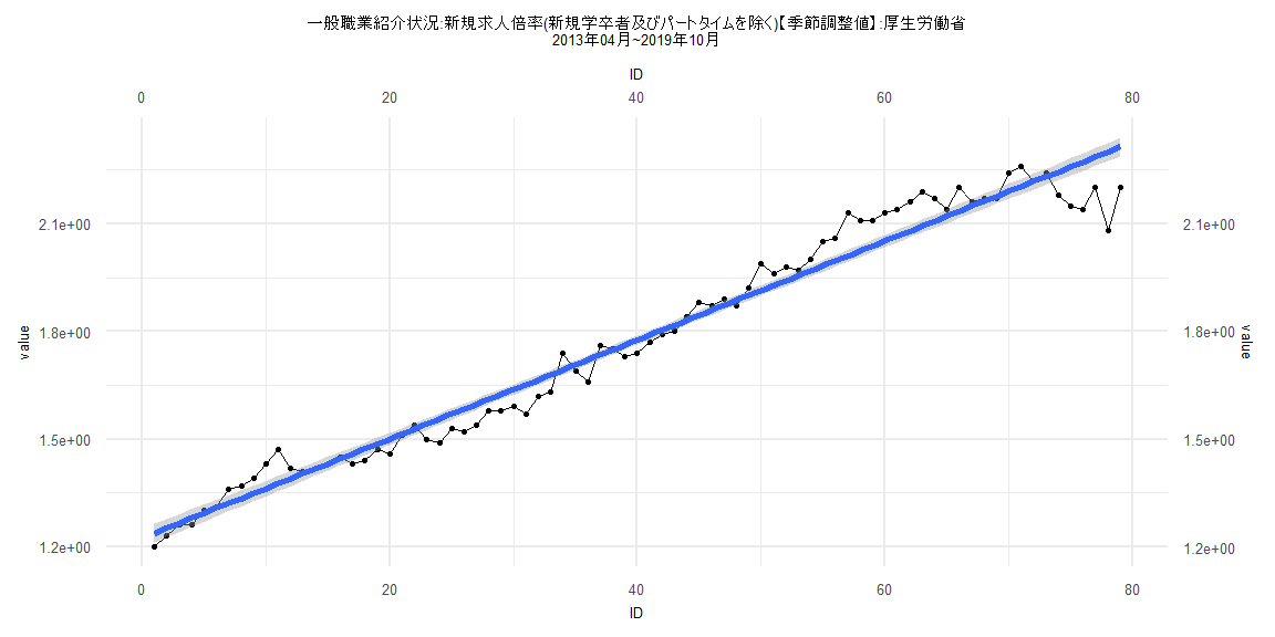
[1] "一般職業紹介状況:新規求人倍率(新規学卒者及びパートタイムを除く)【季節調整値】:厚生労働省"
      Jan  Feb  Mar  Apr  May  Jun  Jul  Aug  Sep  Oct  Nov  Dec
1999                                                        0.75
2000 0.80 0.79 0.79 0.82 0.83 0.85 0.88 0.88 0.89 0.91 0.92 0.92
2001 0.93 0.88 0.84 0.86 0.86 0.83 0.82 0.80 0.77 0.72 0.71 0.69
2002 0.69 0.70 0.72 0.70 0.73 0.74 0.74 0.76 0.75 0.76 0.76 0.80
2003 0.80 0.80 0.82 0.83 0.82 0.82 0.85 0.88 0.89 0.93 0.96 0.98
2004 0.98 0.96 1.01 1.03 1.05 1.10 1.13 1.16 1.21 1.24 1.27 1.28
2005 1.27 1.30 1.28 1.29 1.31 1.31 1.32 1.31 1.31 1.28 1.36 1.37
2006 1.39 1.43 1.39 1.41 1.46 1.42 1.40 1.39 1.39 1.36 1.41 1.43
2007 1.34 1.40 1.44 1.41 1.40 1.37 1.37 1.33 1.25 1.30 1.29 1.25
2008 1.25 1.22 1.14 1.19 1.15 1.12 1.09 1.07 1.02 0.98 0.89 0.82
2009 0.70 0.62 0.62 0.62 0.61 0.63 0.64 0.65 0.67 0.66 0.66 0.67
2010 0.67 0.67 0.67 0.70 0.72 0.73 0.74 0.76 0.79 0.82 0.82 0.84
2011 0.87 0.85 0.81 0.85 0.85 0.87 0.94 0.92 0.99 1.01 1.03 1.03
2012 1.05 1.08 1.04 1.09 1.11 1.12 1.11 1.14 1.10 1.11 1.12 1.13
2013 1.15 1.18 1.17 1.20 1.23 1.26 1.26 1.30 1.31 1.36 1.37 1.39
2014 1.43 1.47 1.42 1.41 1.42 1.43 1.45 1.43 1.44 1.47 1.46 1.51
2015 1.54 1.50 1.49 1.53 1.52 1.54 1.58 1.58 1.59 1.57 1.62 1.63
2016 1.74 1.69 1.66 1.76 1.75 1.73 1.74 1.77 1.79 1.80 1.84 1.88
2017 1.87 1.89 1.87 1.92 1.99 1.96 1.98 1.97 2.00 2.05 2.06 2.13
2018 2.11 2.11 2.13 2.14 2.16 2.19 2.17 2.14 2.20 2.16 2.17 2.17
2019 2.24 2.26 2.22 2.24 2.18 2.15 2.14 2.20 2.08 2.20
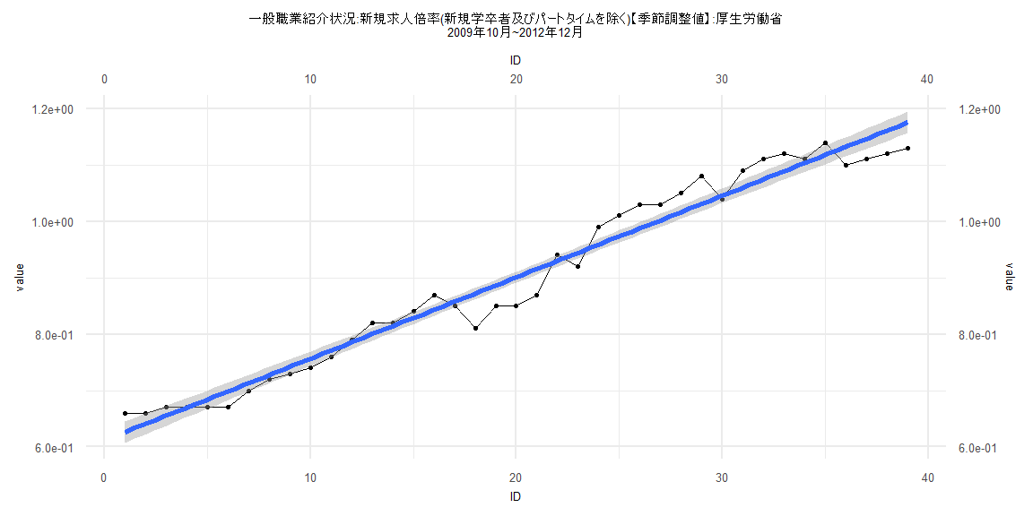
Call:
lm(formula = value ~ ID)

Residuals:
      Min        1Q    Median        3Q       Max
-0.062123 -0.020446  0.004586  0.027297  0.048912

Coefficients:
             Estimate Std. Error t value            Pr(>|t|)
(Intercept) 0.6119973  0.0098501   62.13 <0.0000000000000002 ***
ID          0.0144514  0.0004292   33.67 <0.0000000000000002 ***
---
Signif. codes:  0 '***' 0.001 '**' 0.01 '*' 0.05 '.' 0.1 ' ' 1

Residual standard error: 0.03017 on 37 degrees of freedom
Multiple R-squared:  0.9684,    Adjusted R-squared:  0.9675
F-statistic:  1134 on 1 and 37 DF,  p-value: < 0.00000000000000022


    Two-sample Kolmogorov-Smirnov test

data:  lm_residuals and rnorm(n = length(lm_residuals), mean = 0, sd = sd(lm_residuals))
D = 0.10256, p-value = 0.9885
alternative hypothesis: two-sided


    Durbin-Watson test

data:  value ~ ID
DW = 0.69053, p-value = 0.0000004545
alternative hypothesis: true autocorrelation is greater than 0


    studentized Breusch-Pagan test

data:  value ~ ID
BP = 5.7793, df = 1, p-value = 0.01622


    Box-Ljung test

data:  lm_residuals
X-squared = 15.511, df = 1, p-value = 0.00008202
Call:
lm(formula = value ~ ID)

Residuals:
      Min        1Q    Median        3Q       Max
-0.222961 -0.034078  0.004622  0.037856  0.119008

Coefficients:
             Estimate Std. Error t value            Pr(>|t|)
(Intercept) 1.1767931  0.0127933   91.98 <0.0000000000000002 ***
ID          0.0139033  0.0002678   51.92 <0.0000000000000002 ***
---
Signif. codes:  0 '***' 0.001 '**' 0.01 '*' 0.05 '.' 0.1 ' ' 1

Residual standard error: 0.0574 on 80 degrees of freedom
Multiple R-squared:  0.9712,    Adjusted R-squared:  0.9708
F-statistic:  2696 on 1 and 80 DF,  p-value: < 0.00000000000000022


    Two-sample Kolmogorov-Smirnov test

data:  lm_residuals and rnorm(n = length(lm_residuals), mean = 0, sd = sd(lm_residuals))
D = 0.14634, p-value = 0.3453
alternative hypothesis: two-sided


    Durbin-Watson test

data:  value ~ ID
DW = 0.44229, p-value < 0.00000000000000022
alternative hypothesis: true autocorrelation is greater than 0


    studentized Breusch-Pagan test

data:  value ~ ID
BP = 12.101, df = 1, p-value = 0.000504


    Box-Ljung test

data:  lm_residuals
X-squared = 47.808, df = 1, p-value = 0.000000000004701
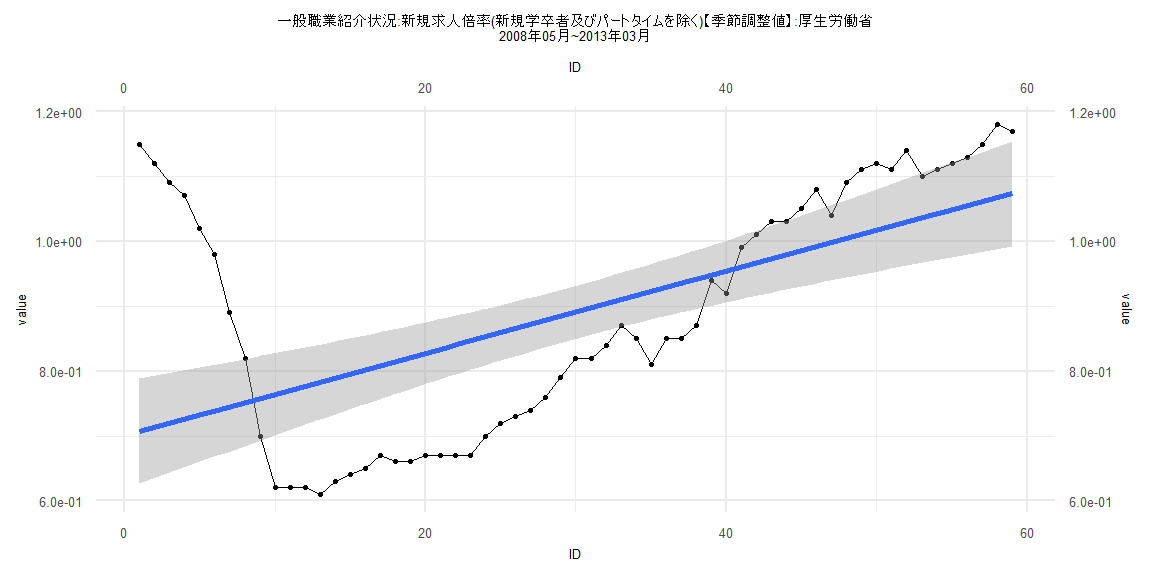
Call:
lm(formula = value ~ ID)

Residuals:
     Min       1Q   Median       3Q      Max
-0.17632 -0.13870 -0.03944  0.08641  0.44254

Coefficients:
            Estimate Std. Error t value             Pr(>|t|)
(Intercept) 0.701146   0.041487  16.900 < 0.0000000000000002 ***
ID          0.006312   0.001203   5.249           0.00000235 ***
---
Signif. codes:  0 '***' 0.001 '**' 0.01 '*' 0.05 '.' 0.1 ' ' 1

Residual standard error: 0.1573 on 57 degrees of freedom
Multiple R-squared:  0.3258,    Adjusted R-squared:  0.314
F-statistic: 27.55 on 1 and 57 DF,  p-value: 0.000002353


    Two-sample Kolmogorov-Smirnov test

data:  lm_residuals and rnorm(n = length(lm_residuals), mean = 0, sd = sd(lm_residuals))
D = 0.15254, p-value = 0.5021
alternative hypothesis: two-sided


    Durbin-Watson test

data:  value ~ ID
DW = 0.052219, p-value < 0.00000000000000022
alternative hypothesis: true autocorrelation is greater than 0


    studentized Breusch-Pagan test

data:  value ~ ID
BP = 21.576, df = 1, p-value = 0.000003401


    Box-Ljung test

data:  lm_residuals
X-squared = 50.393, df = 1, p-value = 0.000000000001258
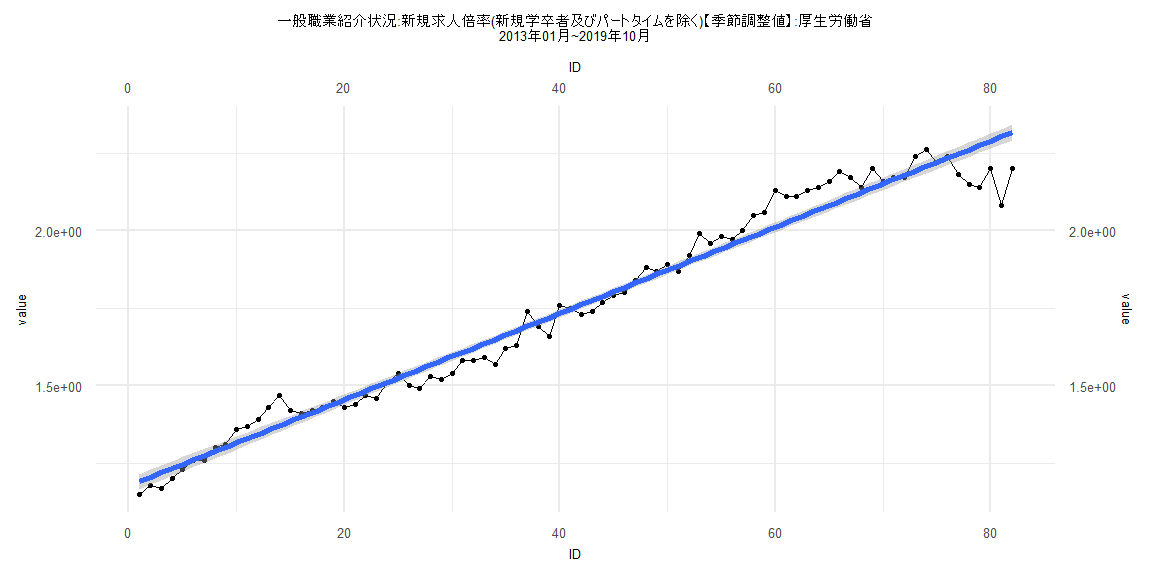
Call:
lm(formula = value ~ ID)

Residuals:
      Min        1Q    Median        3Q       Max
-0.220093 -0.034387  0.002781  0.036823  0.119495

Coefficients:
             Estimate Std. Error t value            Pr(>|t|)
(Intercept) 1.2244791  0.0131556   93.08 <0.0000000000000002 ***
ID          0.0137899  0.0002857   48.26 <0.0000000000000002 ***
---
Signif. codes:  0 '***' 0.001 '**' 0.01 '*' 0.05 '.' 0.1 ' ' 1

Residual standard error: 0.05791 on 77 degrees of freedom
Multiple R-squared:  0.968, Adjusted R-squared:  0.9676
F-statistic:  2329 on 1 and 77 DF,  p-value: < 0.00000000000000022


    Two-sample Kolmogorov-Smirnov test

data:  lm_residuals and rnorm(n = length(lm_residuals), mean = 0, sd = sd(lm_residuals))
D = 0.10127, p-value = 0.8161
alternative hypothesis: two-sided


    Durbin-Watson test

data:  value ~ ID
DW = 0.44709, p-value < 0.00000000000000022
alternative hypothesis: true autocorrelation is greater than 0


    studentized Breusch-Pagan test

data:  value ~ ID
BP = 12.15, df = 1, p-value = 0.0004908


    Box-Ljung test

data:  lm_residuals
X-squared = 45.963, df = 1, p-value = 0.00000000001205