Analysis
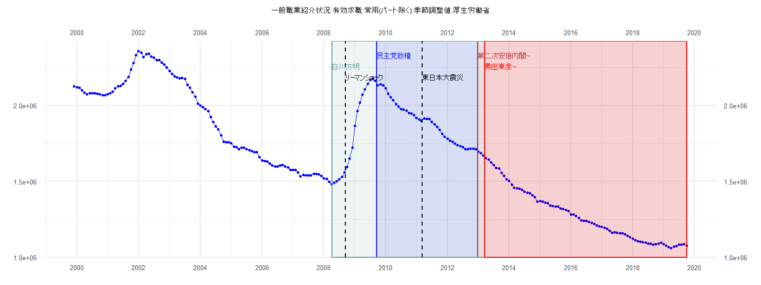
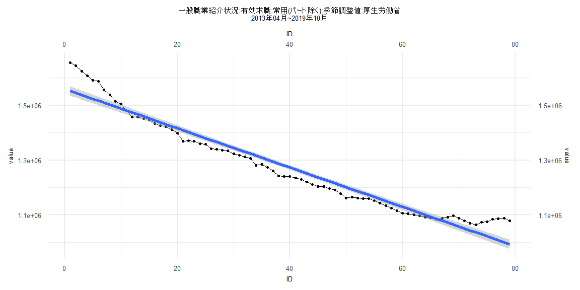
[1] "一般職業紹介状況:有効求職:常用(パート除く):季節調整値:厚生労働省"
         Jan     Feb     Mar     Apr     May     Jun     Jul     Aug     Sep     Oct     Nov     Dec
1999                                                                                         2127092
2000 2118732 2117951 2100634 2083010 2075889 2079553 2079854 2081469 2077344 2074137 2067149 2067791
2001 2072727 2080053 2091448 2113977 2125136 2130111 2142678 2161038 2187647 2236712 2279778 2332842
2002 2357363 2348053 2318717 2337374 2340567 2322406 2315207 2299731 2300454 2283219 2271106 2250803
2003 2228207 2206523 2192396 2185291 2177173 2180336 2176616 2136461 2116330 2087364 2059622 2013003
2004 2001012 1989621 1975699 1963955 1924987 1892091 1864217 1843459 1804898 1762507 1758046 1757266
2005 1750512 1729166 1724321 1713864 1723615 1721378 1712088 1707001 1699524 1694892 1693440 1661076
2006 1639165 1633688 1631355 1619880 1606144 1599514 1600190 1605132 1608163 1600365 1592312 1575856
2007 1577797 1575097 1559092 1535136 1543065 1541413 1541193 1540462 1548587 1549573 1545680 1536475
2008 1520945 1517140 1498383 1482882 1492114 1500479 1514782 1530445 1558562 1594292 1651903 1721180
2009 1864579 1963911 2017916 2070433 2108403 2141156 2168517 2179080 2163227 2133597 2139471 2133968
2010 2112366 2078480 2054647 2034809 2009652 1993322 1976322 1974073 1966538 1951581 1948542 1936836
2011 1916682 1908360 1898836 1914440 1911148 1911859 1890531 1876939 1858216 1839506 1815220 1794711
2012 1782233 1768734 1762504 1749123 1738657 1733696 1726350 1713712 1714170 1716659 1717390 1713443
2013 1698149 1686243 1671631 1655431 1643776 1625101 1608617 1590390 1587189 1555468 1537631 1513807
2014 1505710 1478788 1457503 1457039 1451770 1447080 1432746 1425231 1421837 1410331 1398410 1368785
2015 1370087 1368978 1359720 1357317 1341396 1339363 1336722 1334246 1322448 1317423 1312692 1306603
2016 1281537 1284139 1273269 1259686 1242616 1240793 1240367 1235159 1229202 1220985 1211602 1203700
2017 1202864 1195905 1190205 1177133 1162056 1164479 1161644 1160258 1159761 1151333 1142293 1133795
2018 1123808 1115377 1106606 1104398 1100959 1097767 1091869 1089728 1084829 1088178 1090939 1097062
2019 1087160 1078986 1069422 1063217 1072602 1074822 1084828 1085833 1088001 1077804
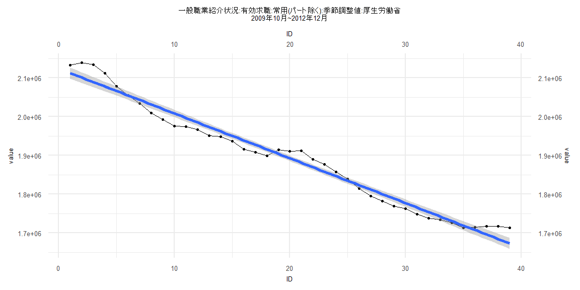
Call:
lm(formula = value ~ ID)

Residuals:
   Min     1Q Median     3Q    Max
-32136 -17506  -8108  18648  44516

Coefficients:
             Estimate Std. Error t value            Pr(>|t|)
(Intercept) 2124163.7     7175.8  296.02 <0.0000000000000002 ***
ID           -11570.6      312.7  -37.01 <0.0000000000000002 ***
---
Signif. codes:  0 '***' 0.001 '**' 0.01 '*' 0.05 '.' 0.1 ' ' 1

Residual standard error: 21980 on 37 degrees of freedom
Multiple R-squared:  0.9737,    Adjusted R-squared:  0.973
F-statistic:  1369 on 1 and 37 DF,  p-value: < 0.00000000000000022


    Two-sample Kolmogorov-Smirnov test

data:  lm_residuals and rnorm(n = length(lm_residuals), mean = 0, sd = sd(lm_residuals))
D = 0.20513, p-value = 0.3888
alternative hypothesis: two-sided


    Durbin-Watson test

data:  value ~ ID
DW = 0.20839, p-value < 0.00000000000000022
alternative hypothesis: true autocorrelation is greater than 0


    studentized Breusch-Pagan test

data:  value ~ ID
BP = 2.4537, df = 1, p-value = 0.1172


    Box-Ljung test

data:  lm_residuals
X-squared = 29.514, df = 1, p-value = 0.00000005551
Call:
lm(formula = value ~ ID)

Residuals:
   Min     1Q Median     3Q    Max
-49817 -29784 -19122  30081 107556

Coefficients:
            Estimate Std. Error t value            Pr(>|t|)
(Intercept)  1598071       9700  164.75 <0.0000000000000002 ***
ID             -7478        203  -36.83 <0.0000000000000002 ***
---
Signif. codes:  0 '***' 0.001 '**' 0.01 '*' 0.05 '.' 0.1 ' ' 1

Residual standard error: 43520 on 80 degrees of freedom
Multiple R-squared:  0.9443,    Adjusted R-squared:  0.9436
F-statistic:  1356 on 1 and 80 DF,  p-value: < 0.00000000000000022


    Two-sample Kolmogorov-Smirnov test

data:  lm_residuals and rnorm(n = length(lm_residuals), mean = 0, sd = sd(lm_residuals))
D = 0.30488, p-value = 0.0009092
alternative hypothesis: two-sided


    Durbin-Watson test

data:  value ~ ID
DW = 0.035605, p-value < 0.00000000000000022
alternative hypothesis: true autocorrelation is greater than 0


    studentized Breusch-Pagan test

data:  value ~ ID
BP = 2.3735, df = 1, p-value = 0.1234


    Box-Ljung test

data:  lm_residuals
X-squared = 71.277, df = 1, p-value < 0.00000000000000022
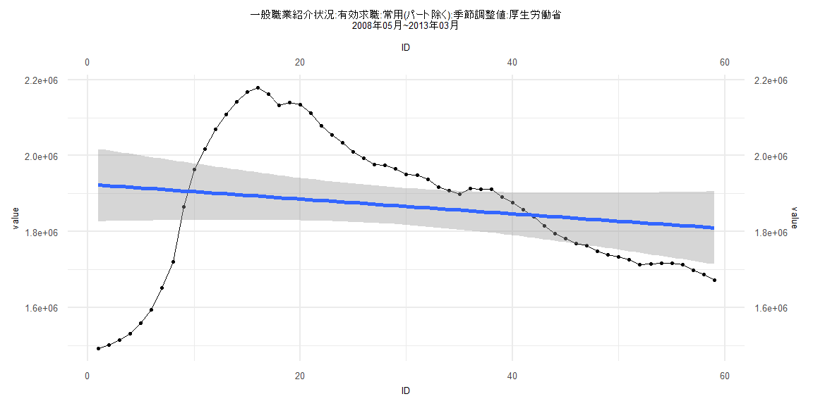
Call:
lm(formula = value ~ ID)

Residuals:
    Min      1Q  Median      3Q     Max
-430600 -101361   41681  116921  285522

Coefficients:
            Estimate Std. Error t value            Pr(>|t|)
(Intercept)  1924658      49054  39.236 <0.0000000000000002 ***
ID             -1944       1422  -1.367               0.177
---
Signif. codes:  0 '***' 0.001 '**' 0.01 '*' 0.05 '.' 0.1 ' ' 1

Residual standard error: 186000 on 57 degrees of freedom
Multiple R-squared:  0.03174,   Adjusted R-squared:  0.01475
F-statistic: 1.869 on 1 and 57 DF,  p-value: 0.177


    Two-sample Kolmogorov-Smirnov test

data:  lm_residuals and rnorm(n = length(lm_residuals), mean = 0, sd = sd(lm_residuals))
D = 0.18644, p-value = 0.2582
alternative hypothesis: two-sided


    Durbin-Watson test

data:  value ~ ID
DW = 0.031023, p-value < 0.00000000000000022
alternative hypothesis: true autocorrelation is greater than 0


    studentized Breusch-Pagan test

data:  value ~ ID
BP = 28.28, df = 1, p-value = 0.000000105


    Box-Ljung test

data:  lm_residuals
X-squared = 53.972, df = 1, p-value = 0.0000000000002034
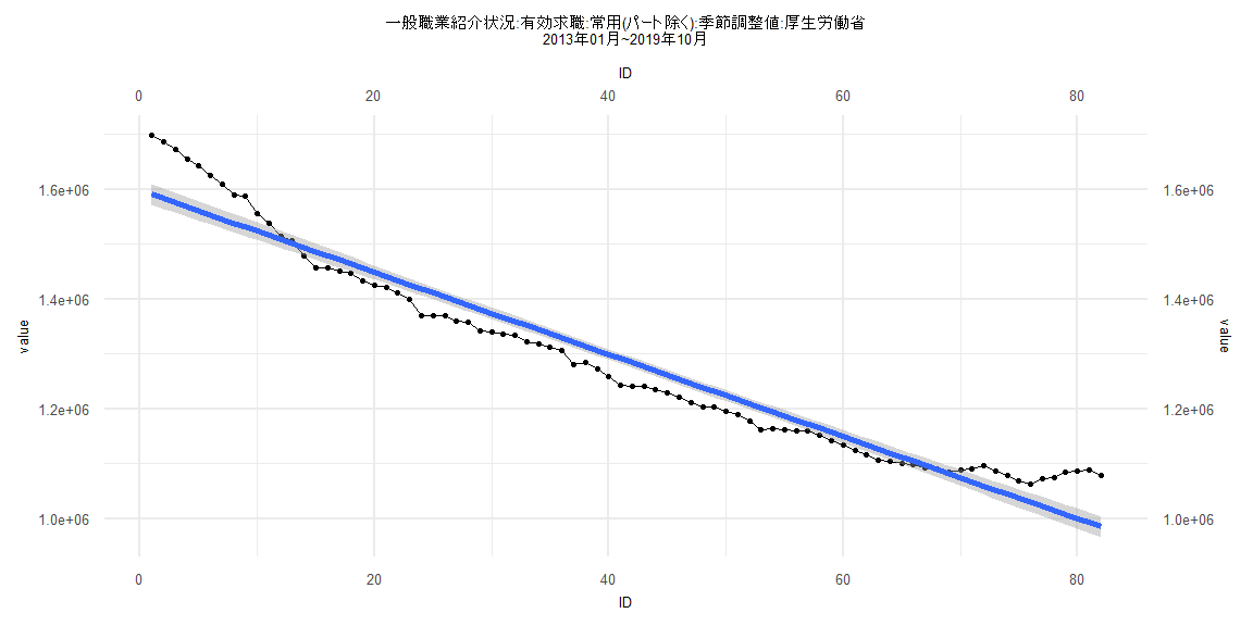
Call:
lm(formula = value ~ ID)

Residuals:
   Min     1Q Median     3Q    Max
-44368 -26521 -15939  18975 103102

Coefficients:
             Estimate Std. Error t value            Pr(>|t|)
(Intercept) 1559500.4     8780.7   177.6 <0.0000000000000002 ***
ID            -7171.5      190.7   -37.6 <0.0000000000000002 ***
---
Signif. codes:  0 '***' 0.001 '**' 0.01 '*' 0.05 '.' 0.1 ' ' 1

Residual standard error: 38650 on 77 degrees of freedom
Multiple R-squared:  0.9484,    Adjusted R-squared:  0.9477
F-statistic:  1414 on 1 and 77 DF,  p-value: < 0.00000000000000022


    Two-sample Kolmogorov-Smirnov test

data:  lm_residuals and rnorm(n = length(lm_residuals), mean = 0, sd = sd(lm_residuals))
D = 0.20253, p-value = 0.07815
alternative hypothesis: two-sided


    Durbin-Watson test

data:  value ~ ID
DW = 0.04565, p-value < 0.00000000000000022
alternative hypothesis: true autocorrelation is greater than 0


    studentized Breusch-Pagan test

data:  value ~ ID
BP = 1.193, df = 1, p-value = 0.2747


    Box-Ljung test

data:  lm_residuals
X-squared = 66.404, df = 1, p-value = 0.0000000000000003331