Analysis
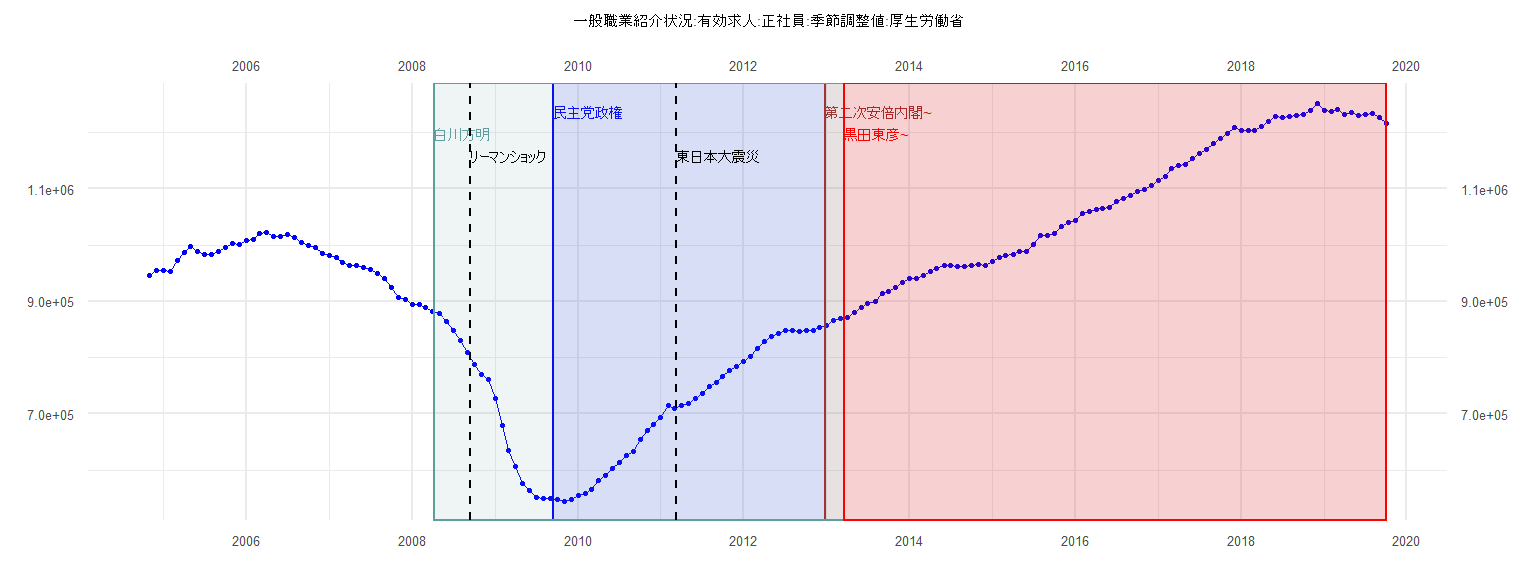
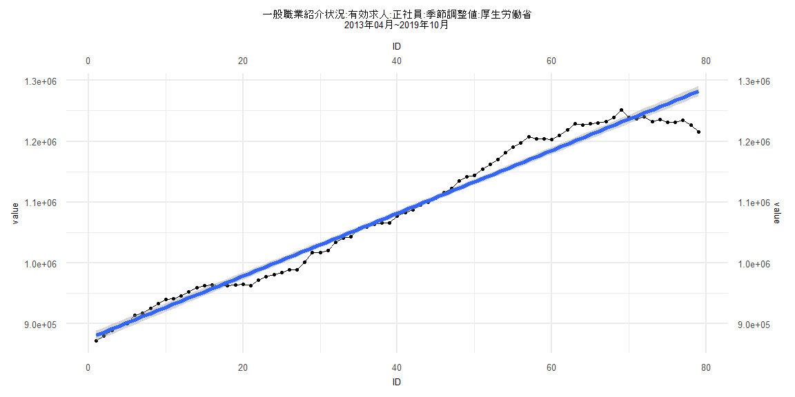
[1] "一般職業紹介状況:有効求人:正社員:季節調整値:厚生労働省"
         Jan     Feb     Mar     Apr     May     Jun     Jul     Aug     Sep     Oct     Nov     Dec
2004                                                                                  946326  954598
2005  955678  953579  973470  986305  997678  989478  983307  982812  987881  996502 1003023 1001328
2006 1008140 1009889 1020053 1021668 1015889 1014791 1019002 1013217 1005324  999655  995428  984605
2007  981590  977603  969473  964041  963211  960154  956146  949849  940830  923817  907741  902767
2008  894595  893749  889358  881970  878737  864661  848033  830434  809697  788636  770686  760790
2009  727807  680232  635896  607127  575776  563380  552371  549095  549615  547802  545337  548952
2010  555038  559427  566107  581147  590254  602938  614646  625392  633661  654570  669854  681164
2011  694364  714191  710121  714704  718154  727576  735506  749589  755136  766783  777187  784395
2012  793077  801863  815752  827947  837198  843849  848062  847931  846823  848659  847630  854409
2013  857902  866129  868850  872215  879827  888950  895776  900269  914115  917728  925382  933832
2014  940404  941053  945634  952474  959080  962887  963534  962804  962521  963514  965473  963111
2015  971737  977452  980658  983754  988972  988636 1001547 1017448 1016981 1021009 1033763 1040511
2016 1042837 1056408 1059016 1063462 1065768 1066365 1076757 1083016 1087364 1095423 1099329 1106684
2017 1115421 1122581 1135512 1142076 1143930 1154635 1162097 1170548 1181051 1190041 1197596 1208051
2018 1204285 1203989 1202984 1209866 1219039 1229044 1226499 1229162 1229954 1231893 1239038 1251417
2019 1239480 1236677 1240260 1232512 1235537 1230996 1231589 1234318 1226413 1215551
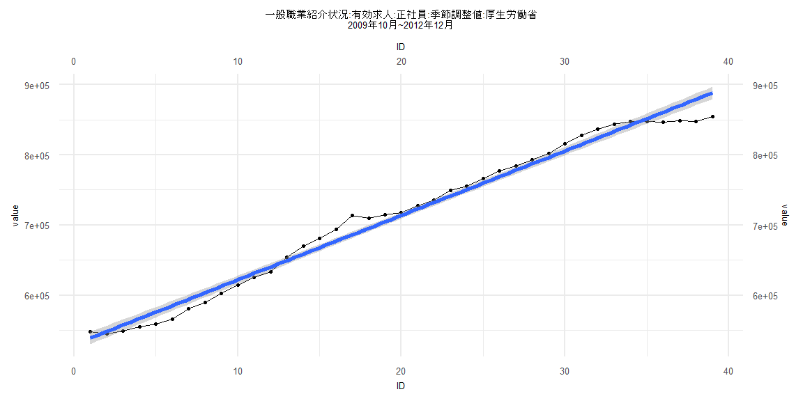
Call:
lm(formula = value ~ ID)

Residuals:
   Min     1Q Median     3Q    Max
-34086  -9088   4606   9384  28004

Coefficients:
            Estimate Std. Error t value            Pr(>|t|)
(Intercept) 529858.1     4490.7  117.99 <0.0000000000000002 ***
ID            9195.8      195.7   46.99 <0.0000000000000002 ***
---
Signif. codes:  0 '***' 0.001 '**' 0.01 '*' 0.05 '.' 0.1 ' ' 1

Residual standard error: 13750 on 37 degrees of freedom
Multiple R-squared:  0.9835,    Adjusted R-squared:  0.9831
F-statistic:  2208 on 1 and 37 DF,  p-value: < 0.00000000000000022


    Two-sample Kolmogorov-Smirnov test

data:  lm_residuals and rnorm(n = length(lm_residuals), mean = 0, sd = sd(lm_residuals))
D = 0.25641, p-value = 0.1547
alternative hypothesis: two-sided


    Durbin-Watson test

data:  value ~ ID
DW = 0.18159, p-value < 0.00000000000000022
alternative hypothesis: true autocorrelation is greater than 0


    studentized Breusch-Pagan test

data:  value ~ ID
BP = 3.443, df = 1, p-value = 0.06352


    Box-Ljung test

data:  lm_residuals
X-squared = 28.345, df = 1, p-value = 0.0000001015
Call:
lm(formula = value ~ ID)

Residuals:
   Min     1Q Median     3Q    Max
-67623  -7732  -1035  12575  38606

Coefficients:
             Estimate Std. Error t value            Pr(>|t|)
(Intercept) 859276.38    4203.16  204.44 <0.0000000000000002 ***
ID            5169.48      87.98   58.76 <0.0000000000000002 ***
---
Signif. codes:  0 '***' 0.001 '**' 0.01 '*' 0.05 '.' 0.1 ' ' 1

Residual standard error: 18860 on 80 degrees of freedom
Multiple R-squared:  0.9774,    Adjusted R-squared:  0.9771
F-statistic:  3453 on 1 and 80 DF,  p-value: < 0.00000000000000022


    Two-sample Kolmogorov-Smirnov test

data:  lm_residuals and rnorm(n = length(lm_residuals), mean = 0, sd = sd(lm_residuals))
D = 0.14634, p-value = 0.3453
alternative hypothesis: two-sided


    Durbin-Watson test

data:  value ~ ID
DW = 0.086076, p-value < 0.00000000000000022
alternative hypothesis: true autocorrelation is greater than 0


    studentized Breusch-Pagan test

data:  value ~ ID
BP = 18.946, df = 1, p-value = 0.00001345


    Box-Ljung test

data:  lm_residuals
X-squared = 65.231, df = 1, p-value = 0.0000000000000006661
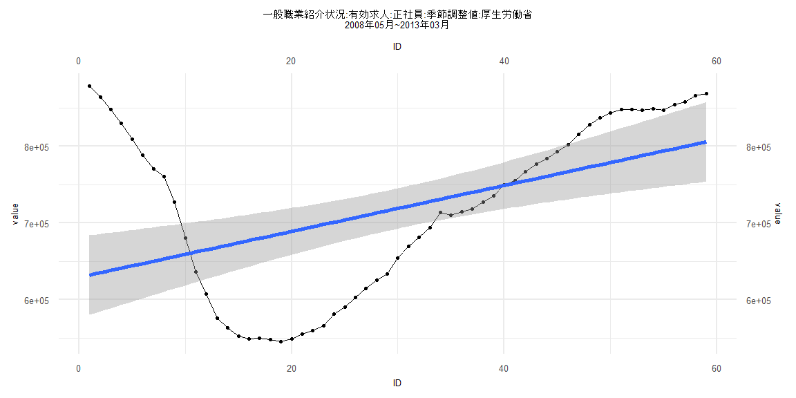
Call:
lm(formula = value ~ ID)

Residuals:
    Min      1Q  Median      3Q     Max
-140739  -89987     592   60055  246593

Coefficients:
            Estimate Std. Error t value             Pr(>|t|)
(Intercept) 629148.2    26601.5  23.651 < 0.0000000000000002 ***
ID            2996.2      771.1   3.885             0.000269 ***
---
Signif. codes:  0 '***' 0.001 '**' 0.01 '*' 0.05 '.' 0.1 ' ' 1

Residual standard error: 100900 on 57 degrees of freedom
Multiple R-squared:  0.2094,    Adjusted R-squared:  0.1955
F-statistic:  15.1 on 1 and 57 DF,  p-value: 0.0002686


    Two-sample Kolmogorov-Smirnov test

data:  lm_residuals and rnorm(n = length(lm_residuals), mean = 0, sd = sd(lm_residuals))
D = 0.11864, p-value = 0.8052
alternative hypothesis: two-sided


    Durbin-Watson test

data:  value ~ ID
DW = 0.023896, p-value < 0.00000000000000022
alternative hypothesis: true autocorrelation is greater than 0


    studentized Breusch-Pagan test

data:  value ~ ID
BP = 26.185, df = 1, p-value = 0.0000003102


    Box-Ljung test

data:  lm_residuals
X-squared = 53.924, df = 1, p-value = 0.0000000000002084
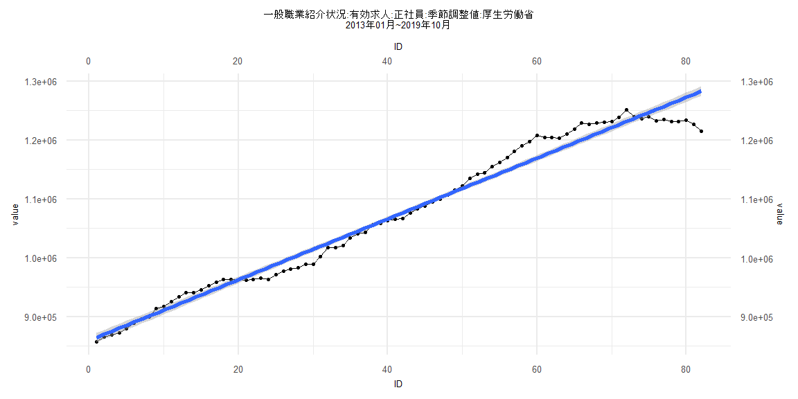
Call:
lm(formula = value ~ ID)

Residuals:
   Min     1Q Median     3Q    Max
-67203  -9296   -850  12745  38675

Coefficients:
             Estimate Std. Error t value            Pr(>|t|)
(Intercept) 875624.86    4358.40  200.91 <0.0000000000000002 ***
ID            5153.53      94.66   54.44 <0.0000000000000002 ***
---
Signif. codes:  0 '***' 0.001 '**' 0.01 '*' 0.05 '.' 0.1 ' ' 1

Residual standard error: 19190 on 77 degrees of freedom
Multiple R-squared:  0.9747,    Adjusted R-squared:  0.9744
F-statistic:  2964 on 1 and 77 DF,  p-value: < 0.00000000000000022


    Two-sample Kolmogorov-Smirnov test

data:  lm_residuals and rnorm(n = length(lm_residuals), mean = 0, sd = sd(lm_residuals))
D = 0.11392, p-value = 0.6878
alternative hypothesis: two-sided


    Durbin-Watson test

data:  value ~ ID
DW = 0.085668, p-value < 0.00000000000000022
alternative hypothesis: true autocorrelation is greater than 0


    studentized Breusch-Pagan test

data:  value ~ ID
BP = 18.024, df = 1, p-value = 0.00002182


    Box-Ljung test

data:  lm_residuals
X-squared = 62.983, df = 1, p-value = 0.000000000000002109