Analysis
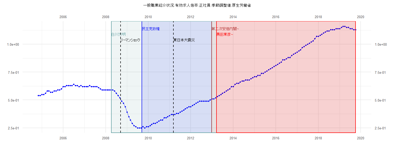
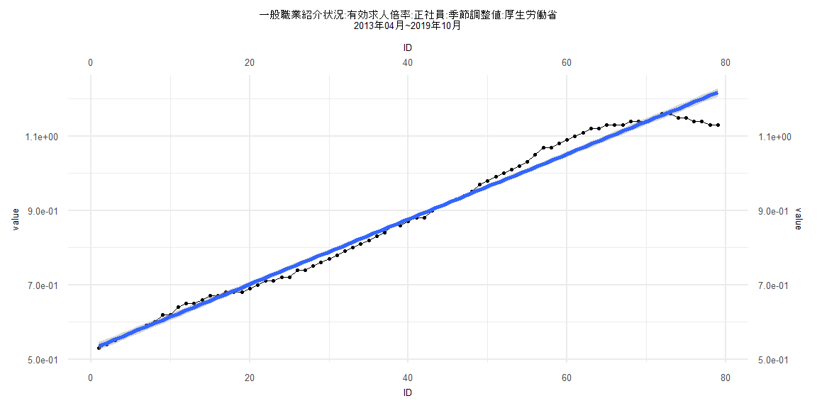
[1] "一般職業紹介状況:有効求人倍率:正社員:季節調整値:厚生労働省"
      Jan  Feb  Mar  Apr  May  Jun  Jul  Aug  Sep  Oct  Nov  Dec
2004                                                   0.54 0.54
2005 0.55 0.55 0.56 0.58 0.58 0.57 0.57 0.58 0.58 0.59 0.59 0.60
2006 0.62 0.62 0.63 0.63 0.63 0.63 0.64 0.63 0.63 0.62 0.63 0.62
2007 0.62 0.62 0.62 0.63 0.62 0.62 0.62 0.62 0.61 0.60 0.59 0.59
2008 0.59 0.59 0.59 0.59 0.59 0.58 0.56 0.54 0.52 0.49 0.47 0.44
2009 0.39 0.35 0.32 0.29 0.27 0.26 0.25 0.25 0.25 0.26 0.25 0.26
2010 0.26 0.27 0.28 0.29 0.29 0.30 0.31 0.32 0.32 0.34 0.34 0.35
2011 0.36 0.37 0.37 0.37 0.38 0.38 0.39 0.40 0.41 0.42 0.43 0.44
2012 0.44 0.45 0.46 0.47 0.48 0.49 0.49 0.49 0.49 0.49 0.49 0.50
2013 0.51 0.51 0.52 0.53 0.54 0.55 0.56 0.57 0.58 0.59 0.60 0.62
2014 0.62 0.64 0.65 0.65 0.66 0.67 0.67 0.68 0.68 0.68 0.69 0.70
2015 0.71 0.71 0.72 0.72 0.74 0.74 0.75 0.76 0.77 0.78 0.79 0.80
2016 0.81 0.82 0.83 0.84 0.86 0.86 0.87 0.88 0.88 0.90 0.91 0.92
2017 0.93 0.94 0.95 0.97 0.98 0.99 1.00 1.01 1.02 1.03 1.05 1.07
2018 1.07 1.08 1.09 1.10 1.11 1.12 1.12 1.13 1.13 1.13 1.14 1.14
2019 1.14 1.15 1.16 1.16 1.15 1.15 1.14 1.14 1.13 1.13
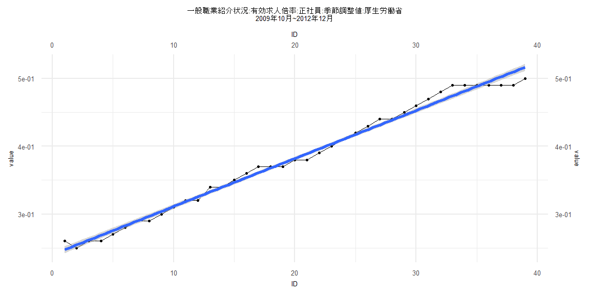
Call:
lm(formula = value ~ ID)

Residuals:
       Min         1Q     Median         3Q        Max
-0.0196545 -0.0051505  0.0001066  0.0058596  0.0157908

Coefficients:
            Estimate Std. Error t value            Pr(>|t|)
(Intercept) 0.240270   0.002617   91.81 <0.0000000000000002 ***
ID          0.007089   0.000114   62.17 <0.0000000000000002 ***
---
Signif. codes:  0 '***' 0.001 '**' 0.01 '*' 0.05 '.' 0.1 ' ' 1

Residual standard error: 0.008015 on 37 degrees of freedom
Multiple R-squared:  0.9905,    Adjusted R-squared:  0.9903
F-statistic:  3865 on 1 and 37 DF,  p-value: < 0.00000000000000022


    Two-sample Kolmogorov-Smirnov test

data:  lm_residuals and rnorm(n = length(lm_residuals), mean = 0, sd = sd(lm_residuals))
D = 0.12821, p-value = 0.9114
alternative hypothesis: two-sided


    Durbin-Watson test

data:  value ~ ID
DW = 0.54989, p-value = 0.00000000809
alternative hypothesis: true autocorrelation is greater than 0


    studentized Breusch-Pagan test

data:  value ~ ID
BP = 8.3889, df = 1, p-value = 0.003775


    Box-Ljung test

data:  lm_residuals
X-squared = 16.832, df = 1, p-value = 0.00004084
Call:
lm(formula = value ~ ID)

Residuals:
      Min        1Q    Median        3Q       Max
-0.088290 -0.012121  0.000473  0.015751  0.044548

Coefficients:
             Estimate Std. Error t value            Pr(>|t|)
(Intercept) 0.4995303  0.0054218   92.13 <0.0000000000000002 ***
ID          0.0087654  0.0001135   77.24 <0.0000000000000002 ***
---
Signif. codes:  0 '***' 0.001 '**' 0.01 '*' 0.05 '.' 0.1 ' ' 1

Residual standard error: 0.02432 on 80 degrees of freedom
Multiple R-squared:  0.9868,    Adjusted R-squared:  0.9866
F-statistic:  5966 on 1 and 80 DF,  p-value: < 0.00000000000000022


    Two-sample Kolmogorov-Smirnov test

data:  lm_residuals and rnorm(n = length(lm_residuals), mean = 0, sd = sd(lm_residuals))
D = 0.14634, p-value = 0.3453
alternative hypothesis: two-sided


    Durbin-Watson test

data:  value ~ ID
DW = 0.079318, p-value < 0.00000000000000022
alternative hypothesis: true autocorrelation is greater than 0


    studentized Breusch-Pagan test

data:  value ~ ID
BP = 20.078, df = 1, p-value = 0.000007434


    Box-Ljung test

data:  lm_residuals
X-squared = 65.549, df = 1, p-value = 0.0000000000000005551
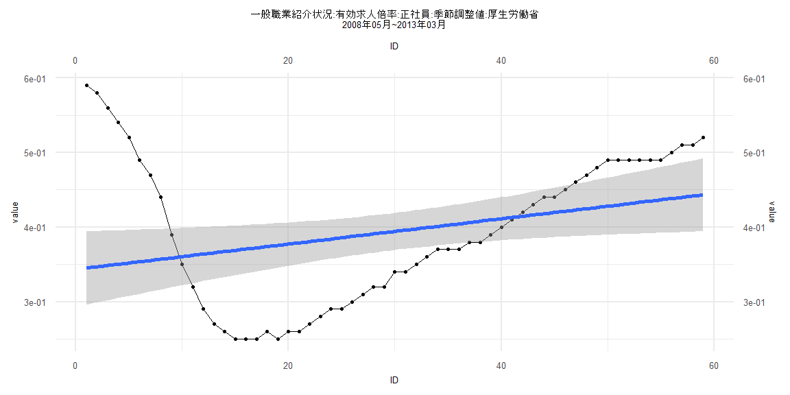
Call:
lm(formula = value ~ ID)

Residuals:
     Min       1Q   Median       3Q      Max
-0.12562 -0.07647 -0.01116  0.05769  0.24483

Coefficients:
             Estimate Std. Error t value            Pr(>|t|)
(Intercept) 0.3434775  0.0251566   13.65 <0.0000000000000002 ***
ID          0.0016920  0.0007293    2.32              0.0239 *
---
Signif. codes:  0 '***' 0.001 '**' 0.01 '*' 0.05 '.' 0.1 ' ' 1

Residual standard error: 0.09539 on 57 degrees of freedom
Multiple R-squared:  0.08629,   Adjusted R-squared:  0.07026
F-statistic: 5.383 on 1 and 57 DF,  p-value: 0.02393


    Two-sample Kolmogorov-Smirnov test

data:  lm_residuals and rnorm(n = length(lm_residuals), mean = 0, sd = sd(lm_residuals))
D = 0.11864, p-value = 0.8052
alternative hypothesis: two-sided


    Durbin-Watson test

data:  value ~ ID
DW = 0.026034, p-value < 0.00000000000000022
alternative hypothesis: true autocorrelation is greater than 0


    studentized Breusch-Pagan test

data:  value ~ ID
BP = 23.441, df = 1, p-value = 0.000001288


    Box-Ljung test

data:  lm_residuals
X-squared = 52.924, df = 1, p-value = 0.0000000000003467
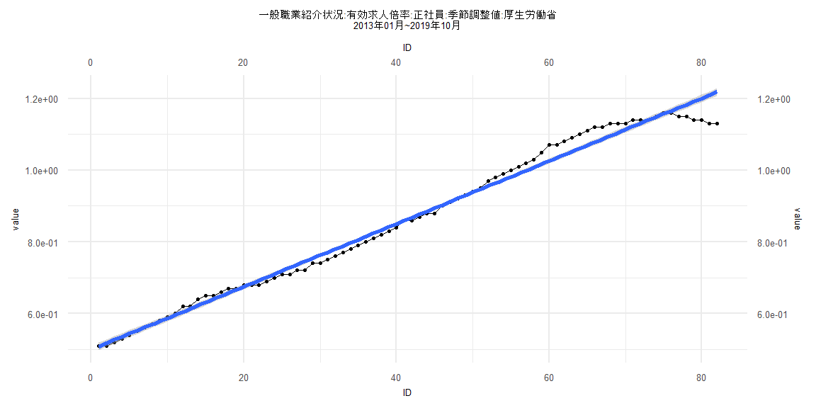
Call:
lm(formula = value ~ ID)

Residuals:
      Min        1Q    Median        3Q       Max
-0.088003 -0.012775  0.000786  0.016462  0.044593

Coefficients:
             Estimate Std. Error t value            Pr(>|t|)
(Intercept) 0.5264070  0.0056267   93.55 <0.0000000000000002 ***
ID          0.0087544  0.0001222   71.64 <0.0000000000000002 ***
---
Signif. codes:  0 '***' 0.001 '**' 0.01 '*' 0.05 '.' 0.1 ' ' 1

Residual standard error: 0.02477 on 77 degrees of freedom
Multiple R-squared:  0.9852,    Adjusted R-squared:  0.985
F-statistic:  5132 on 1 and 77 DF,  p-value: < 0.00000000000000022


    Two-sample Kolmogorov-Smirnov test

data:  lm_residuals and rnorm(n = length(lm_residuals), mean = 0, sd = sd(lm_residuals))
D = 0.16456, p-value = 0.2361
alternative hypothesis: two-sided


    Durbin-Watson test

data:  value ~ ID
DW = 0.077745, p-value < 0.00000000000000022
alternative hypothesis: true autocorrelation is greater than 0


    studentized Breusch-Pagan test

data:  value ~ ID
BP = 19.429, df = 1, p-value = 0.00001044


    Box-Ljung test

data:  lm_residuals
X-squared = 63.368, df = 1, p-value = 0.000000000000001665