Analysis
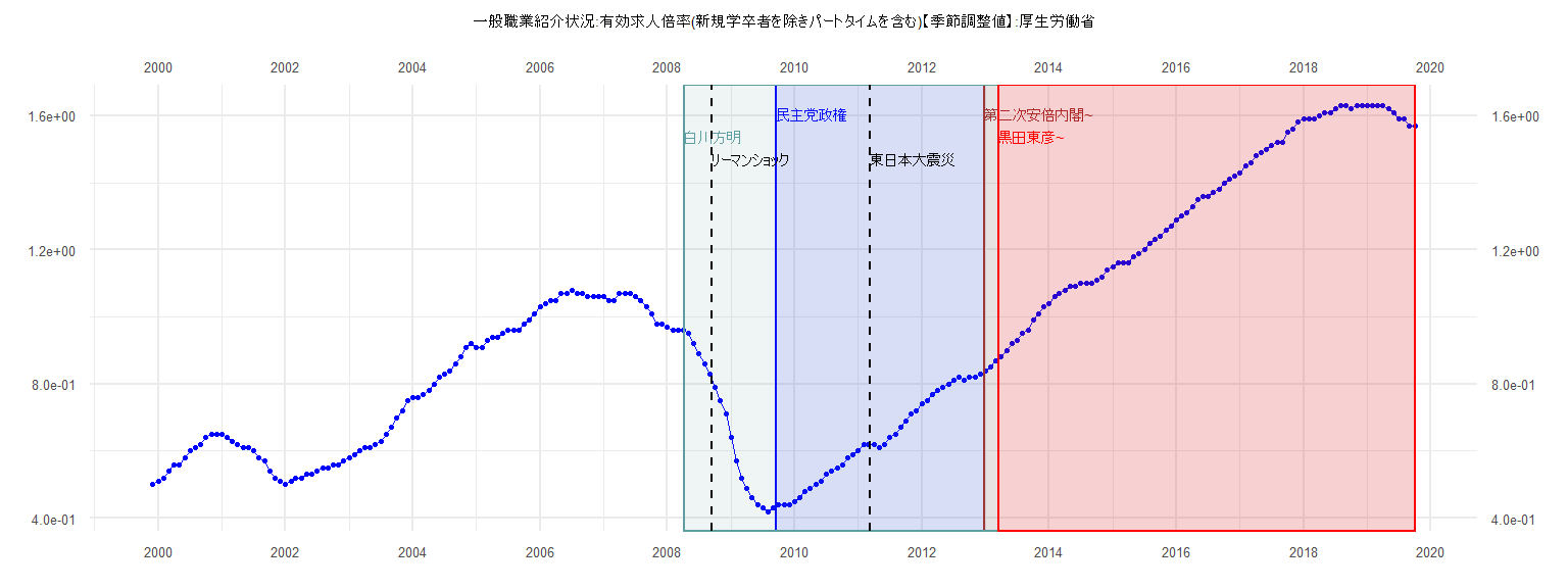
[1] "一般職業紹介状況:有効求人倍率(新規学卒者を除きパートタイムを含む)【季節調整値】:厚生労働省"
      Jan  Feb  Mar  Apr  May  Jun  Jul  Aug  Sep  Oct  Nov  Dec
1999                                                        0.50
2000 0.51 0.52 0.54 0.56 0.56 0.58 0.60 0.61 0.62 0.64 0.65 0.65
2001 0.65 0.64 0.63 0.62 0.61 0.61 0.60 0.58 0.57 0.54 0.52 0.51
2002 0.50 0.51 0.52 0.52 0.53 0.53 0.54 0.55 0.55 0.56 0.56 0.57
2003 0.58 0.59 0.60 0.61 0.61 0.62 0.63 0.65 0.67 0.70 0.72 0.75
2004 0.76 0.76 0.77 0.78 0.80 0.82 0.83 0.84 0.86 0.88 0.91 0.92
2005 0.91 0.91 0.93 0.94 0.94 0.95 0.96 0.96 0.96 0.98 0.99 1.01
2006 1.03 1.04 1.05 1.05 1.07 1.07 1.08 1.07 1.07 1.06 1.06 1.06
2007 1.06 1.05 1.05 1.07 1.07 1.07 1.06 1.05 1.03 1.01 0.98 0.98
2008 0.97 0.96 0.96 0.96 0.95 0.92 0.89 0.86 0.83 0.79 0.75 0.71
2009 0.64 0.57 0.52 0.49 0.46 0.44 0.43 0.42 0.43 0.44 0.44 0.44
2010 0.45 0.46 0.48 0.49 0.50 0.51 0.53 0.54 0.55 0.56 0.58 0.59
2011 0.60 0.62 0.62 0.62 0.61 0.62 0.64 0.65 0.67 0.69 0.71 0.72
2012 0.74 0.75 0.77 0.78 0.79 0.80 0.81 0.82 0.81 0.82 0.82 0.83
2013 0.84 0.85 0.87 0.88 0.90 0.92 0.93 0.95 0.96 0.99 1.01 1.03
2014 1.04 1.06 1.07 1.08 1.09 1.09 1.10 1.10 1.10 1.11 1.12 1.14
2015 1.15 1.16 1.16 1.16 1.18 1.19 1.20 1.22 1.23 1.24 1.26 1.27
2016 1.29 1.30 1.31 1.33 1.35 1.36 1.36 1.37 1.38 1.40 1.41 1.42
2017 1.43 1.45 1.46 1.48 1.49 1.50 1.51 1.52 1.52 1.55 1.56 1.58
2018 1.59 1.59 1.59 1.60 1.61 1.61 1.62 1.63 1.63 1.62 1.63 1.63
2019 1.63 1.63 1.63 1.63 1.62 1.61 1.59 1.59 1.57 1.57
Call:
lm(formula = value ~ ID)

Residuals:
      Min        1Q    Median        3Q       Max
-0.028945 -0.007692  0.002332  0.010428  0.019777

Coefficients:
            Estimate Std. Error t value            Pr(>|t|)
(Intercept) 0.412632   0.004406   93.66 <0.0000000000000002 ***
ID          0.011253   0.000192   58.62 <0.0000000000000002 ***
---
Signif. codes:  0 '***' 0.001 '**' 0.01 '*' 0.05 '.' 0.1 ' ' 1

Residual standard error: 0.01349 on 37 degrees of freedom
Multiple R-squared:  0.9893,    Adjusted R-squared:  0.9891
F-statistic:  3436 on 1 and 37 DF,  p-value: < 0.00000000000000022


    Two-sample Kolmogorov-Smirnov test

data:  lm_residuals and rnorm(n = length(lm_residuals), mean = 0, sd = sd(lm_residuals))
D = 0.076923, p-value = 0.9999
alternative hypothesis: two-sided


    Durbin-Watson test

data:  value ~ ID
DW = 0.34659, p-value = 0.00000000000133
alternative hypothesis: true autocorrelation is greater than 0


    studentized Breusch-Pagan test

data:  value ~ ID
BP = 5.6803, df = 1, p-value = 0.01716


    Box-Ljung test

data:  lm_residuals
X-squared = 25.151, df = 1, p-value = 0.0000005301
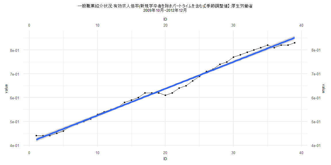
Call:
lm(formula = value ~ ID)

Residuals:
      Min        1Q    Median        3Q       Max
-0.168310 -0.013936  0.007207  0.032628  0.067860

Coefficients:
             Estimate Std. Error t value            Pr(>|t|)
(Intercept) 0.8953117  0.0106177   84.32 <0.0000000000000002 ***
ID          0.0102805  0.0002222   46.26 <0.0000000000000002 ***
---
Signif. codes:  0 '***' 0.001 '**' 0.01 '*' 0.05 '.' 0.1 ' ' 1

Residual standard error: 0.04763 on 80 degrees of freedom
Multiple R-squared:  0.964, Adjusted R-squared:  0.9635
F-statistic:  2140 on 1 and 80 DF,  p-value: < 0.00000000000000022


    Two-sample Kolmogorov-Smirnov test

data:  lm_residuals and rnorm(n = length(lm_residuals), mean = 0, sd = sd(lm_residuals))
D = 0.12195, p-value = 0.5785
alternative hypothesis: two-sided


    Durbin-Watson test

data:  value ~ ID
DW = 0.041048, p-value < 0.00000000000000022
alternative hypothesis: true autocorrelation is greater than 0


    studentized Breusch-Pagan test

data:  value ~ ID
BP = 14.699, df = 1, p-value = 0.0001261


    Box-Ljung test

data:  lm_residuals
X-squared = 67.297, df = 1, p-value = 0.000000000000000222
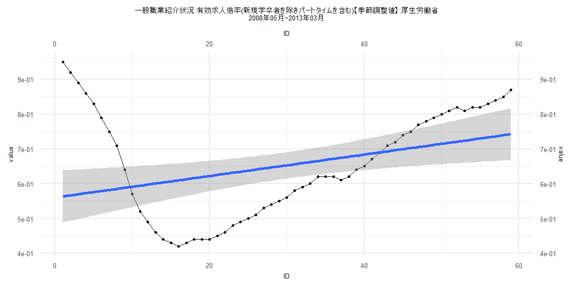
Call:
lm(formula = value ~ ID)

Residuals:
     Min       1Q   Median       3Q      Max
-0.18986 -0.11065 -0.03390  0.09099  0.38642

Coefficients:
            Estimate Std. Error t value             Pr(>|t|)
(Intercept) 0.560491   0.038398  14.597 < 0.0000000000000002 ***
ID          0.003085   0.001113   2.772              0.00752 **
---
Signif. codes:  0 '***' 0.001 '**' 0.01 '*' 0.05 '.' 0.1 ' ' 1

Residual standard error: 0.1456 on 57 degrees of freedom
Multiple R-squared:  0.1188,    Adjusted R-squared:  0.1033
F-statistic: 7.683 on 1 and 57 DF,  p-value: 0.007517


    Two-sample Kolmogorov-Smirnov test

data:  lm_residuals and rnorm(n = length(lm_residuals), mean = 0, sd = sd(lm_residuals))
D = 0.10169, p-value = 0.9239
alternative hypothesis: two-sided


    Durbin-Watson test

data:  value ~ ID
DW = 0.025858, p-value < 0.00000000000000022
alternative hypothesis: true autocorrelation is greater than 0


    studentized Breusch-Pagan test

data:  value ~ ID
BP = 22.327, df = 1, p-value = 0.0000023


    Box-Ljung test

data:  lm_residuals
X-squared = 52.356, df = 1, p-value = 0.0000000000004629
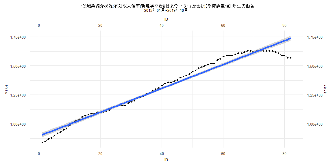
Call:
lm(formula = value ~ ID)

Residuals:
      Min        1Q    Median        3Q       Max
-0.163373 -0.018073  0.003136  0.030393  0.068672

Coefficients:
             Estimate Std. Error t value            Pr(>|t|)
(Intercept) 0.9360273  0.0106061   88.25 <0.0000000000000002 ***
ID          0.0100930  0.0002303   43.82 <0.0000000000000002 ***
---
Signif. codes:  0 '***' 0.001 '**' 0.01 '*' 0.05 '.' 0.1 ' ' 1

Residual standard error: 0.04669 on 77 degrees of freedom
Multiple R-squared:  0.9614,    Adjusted R-squared:  0.9609
F-statistic:  1920 on 1 and 77 DF,  p-value: < 0.00000000000000022


    Two-sample Kolmogorov-Smirnov test

data:  lm_residuals and rnorm(n = length(lm_residuals), mean = 0, sd = sd(lm_residuals))
D = 0.13924, p-value = 0.4302
alternative hypothesis: two-sided


    Durbin-Watson test

data:  value ~ ID
DW = 0.043598, p-value < 0.00000000000000022
alternative hypothesis: true autocorrelation is greater than 0


    studentized Breusch-Pagan test

data:  value ~ ID
BP = 16.176, df = 1, p-value = 0.00005773


    Box-Ljung test

data:  lm_residuals
X-squared = 64.351, df = 1, p-value = 0.0000000000000009992