Analysis
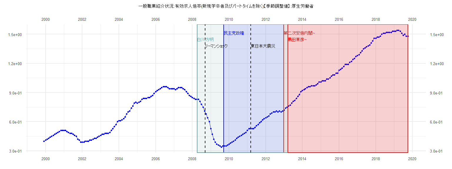
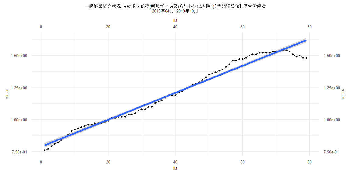
[1] "一般職業紹介状況:有効求人倍率(新規学卒者及びパートタイムを除く)【季節調整値】:厚生労働省"
      Jan  Feb  Mar  Apr  May  Jun  Jul  Aug  Sep  Oct  Nov  Dec
1999                                                        0.40
2000 0.41 0.42 0.43 0.44 0.45 0.46 0.47 0.48 0.49 0.50 0.51 0.51
2001 0.51 0.51 0.50 0.49 0.48 0.48 0.47 0.46 0.45 0.42 0.41 0.39
2002 0.39 0.39 0.40 0.40 0.40 0.41 0.41 0.42 0.43 0.43 0.44 0.45
2003 0.46 0.47 0.47 0.48 0.48 0.48 0.49 0.51 0.53 0.55 0.57 0.60
2004 0.61 0.61 0.62 0.63 0.65 0.68 0.70 0.71 0.74 0.76 0.79 0.80
2005 0.79 0.80 0.81 0.83 0.84 0.84 0.84 0.85 0.85 0.86 0.87 0.89
2006 0.91 0.92 0.93 0.94 0.95 0.96 0.96 0.96 0.95 0.94 0.94 0.94
2007 0.94 0.93 0.94 0.95 0.95 0.95 0.94 0.93 0.91 0.89 0.87 0.86
2008 0.85 0.84 0.83 0.83 0.83 0.81 0.78 0.75 0.71 0.68 0.64 0.60
2009 0.53 0.47 0.42 0.39 0.37 0.36 0.35 0.34 0.35 0.35 0.35 0.36
2010 0.37 0.38 0.39 0.40 0.41 0.43 0.44 0.45 0.46 0.47 0.48 0.49
2011 0.51 0.53 0.53 0.53 0.53 0.54 0.56 0.57 0.59 0.60 0.62 0.63
2012 0.64 0.65 0.66 0.68 0.69 0.70 0.70 0.71 0.70 0.71 0.70 0.71
2013 0.72 0.74 0.75 0.76 0.77 0.79 0.81 0.82 0.84 0.86 0.88 0.91
2014 0.92 0.93 0.94 0.95 0.96 0.96 0.97 0.97 0.97 0.98 0.99 1.01
2015 1.01 1.02 1.02 1.02 1.04 1.04 1.05 1.07 1.08 1.08 1.10 1.10
2016 1.13 1.14 1.15 1.17 1.19 1.19 1.19 1.21 1.22 1.24 1.25 1.27
2017 1.28 1.29 1.31 1.33 1.35 1.36 1.37 1.38 1.39 1.41 1.43 1.46
2018 1.46 1.47 1.47 1.48 1.50 1.51 1.51 1.52 1.52 1.52 1.52 1.53
2019 1.53 1.53 1.54 1.54 1.53 1.51 1.49 1.50 1.48 1.48
Call:
lm(formula = value ~ ID)

Residuals:
      Min        1Q    Median        3Q       Max
-0.034603 -0.005787  0.000318  0.008134  0.019818

Coefficients:
             Estimate Std. Error t value            Pr(>|t|)
(Intercept) 0.3330499  0.0041003   81.22 <0.0000000000000002 ***
ID          0.0105526  0.0001787   59.06 <0.0000000000000002 ***
---
Signif. codes:  0 '***' 0.001 '**' 0.01 '*' 0.05 '.' 0.1 ' ' 1

Residual standard error: 0.01256 on 37 degrees of freedom
Multiple R-squared:  0.9895,    Adjusted R-squared:  0.9892
F-statistic:  3488 on 1 and 37 DF,  p-value: < 0.00000000000000022


    Two-sample Kolmogorov-Smirnov test

data:  lm_residuals and rnorm(n = length(lm_residuals), mean = 0, sd = sd(lm_residuals))
D = 0.15385, p-value = 0.7523
alternative hypothesis: two-sided


    Durbin-Watson test

data:  value ~ ID
DW = 0.34854, p-value = 0.000000000001485
alternative hypothesis: true autocorrelation is greater than 0


    studentized Breusch-Pagan test

data:  value ~ ID
BP = 12.263, df = 1, p-value = 0.0004621


    Box-Ljung test

data:  lm_residuals
X-squared = 21.791, df = 1, p-value = 0.000003041
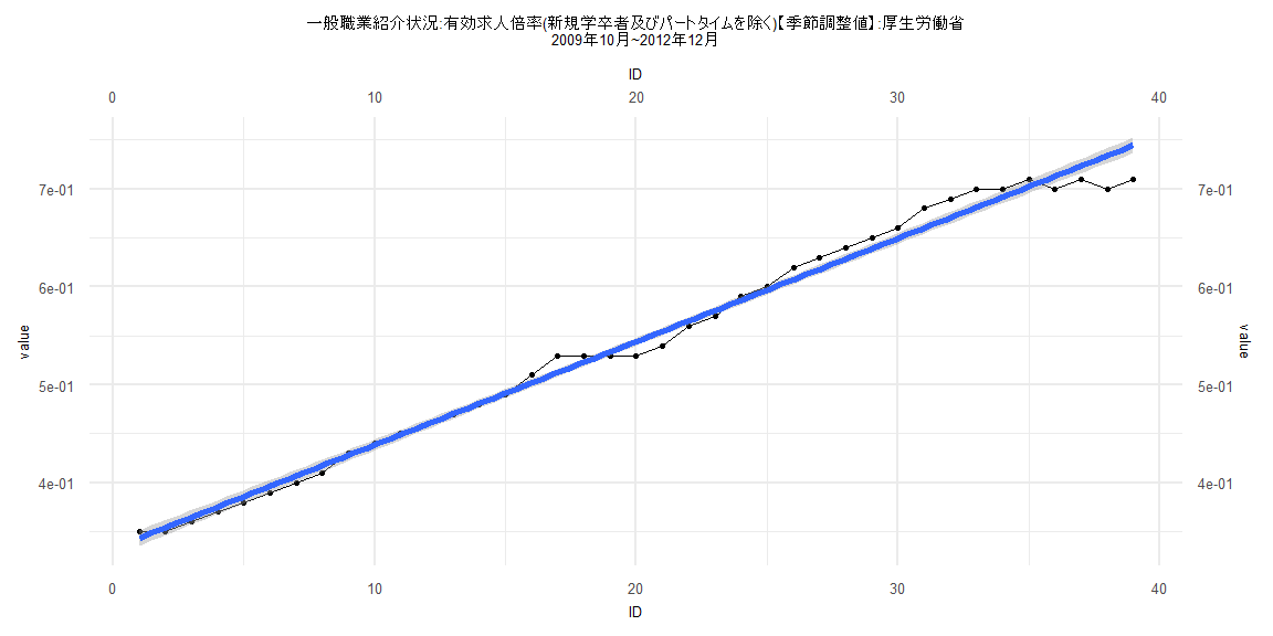
Call:
lm(formula = value ~ ID)

Residuals:
      Min        1Q    Median        3Q       Max
-0.141825 -0.018245 -0.001478  0.030377  0.072084

Coefficients:
             Estimate Std. Error t value            Pr(>|t|)
(Intercept) 0.7499819  0.0089495   83.80 <0.0000000000000002 ***
ID          0.0106322  0.0001873   56.76 <0.0000000000000002 ***
---
Signif. codes:  0 '***' 0.001 '**' 0.01 '*' 0.05 '.' 0.1 ' ' 1

Residual standard error: 0.04015 on 80 degrees of freedom
Multiple R-squared:  0.9758,    Adjusted R-squared:  0.9755
F-statistic:  3222 on 1 and 80 DF,  p-value: < 0.00000000000000022


    Two-sample Kolmogorov-Smirnov test

data:  lm_residuals and rnorm(n = length(lm_residuals), mean = 0, sd = sd(lm_residuals))
D = 0.17073, p-value = 0.1836
alternative hypothesis: two-sided


    Durbin-Watson test

data:  value ~ ID
DW = 0.066651, p-value < 0.00000000000000022
alternative hypothesis: true autocorrelation is greater than 0


    studentized Breusch-Pagan test

data:  value ~ ID
BP = 17.075, df = 1, p-value = 0.00003593


    Box-Ljung test

data:  lm_residuals
X-squared = 66.197, df = 1, p-value = 0.0000000000000004441
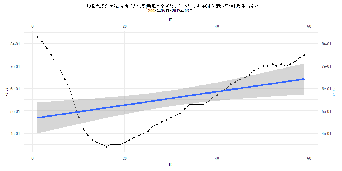
Call:
lm(formula = value ~ ID)

Residuals:
     Min       1Q   Median       3Q      Max
-0.17426 -0.10972 -0.02300  0.07912  0.36058

Coefficients:
            Estimate Std. Error t value            Pr(>|t|)
(Intercept) 0.466435   0.035642  13.086 <0.0000000000000002 ***
ID          0.002989   0.001033   2.893              0.0054 **
---
Signif. codes:  0 '***' 0.001 '**' 0.01 '*' 0.05 '.' 0.1 ' ' 1

Residual standard error: 0.1352 on 57 degrees of freedom
Multiple R-squared:  0.128, Adjusted R-squared:  0.1127
F-statistic: 8.368 on 1 and 57 DF,  p-value: 0.005399


    Two-sample Kolmogorov-Smirnov test

data:  lm_residuals and rnorm(n = length(lm_residuals), mean = 0, sd = sd(lm_residuals))
D = 0.15254, p-value = 0.5021
alternative hypothesis: two-sided


    Durbin-Watson test

data:  value ~ ID
DW = 0.026506, p-value < 0.00000000000000022
alternative hypothesis: true autocorrelation is greater than 0


    studentized Breusch-Pagan test

data:  value ~ ID
BP = 22.788, df = 1, p-value = 0.000001809


    Box-Ljung test

data:  lm_residuals
X-squared = 52.382, df = 1, p-value = 0.0000000000004569
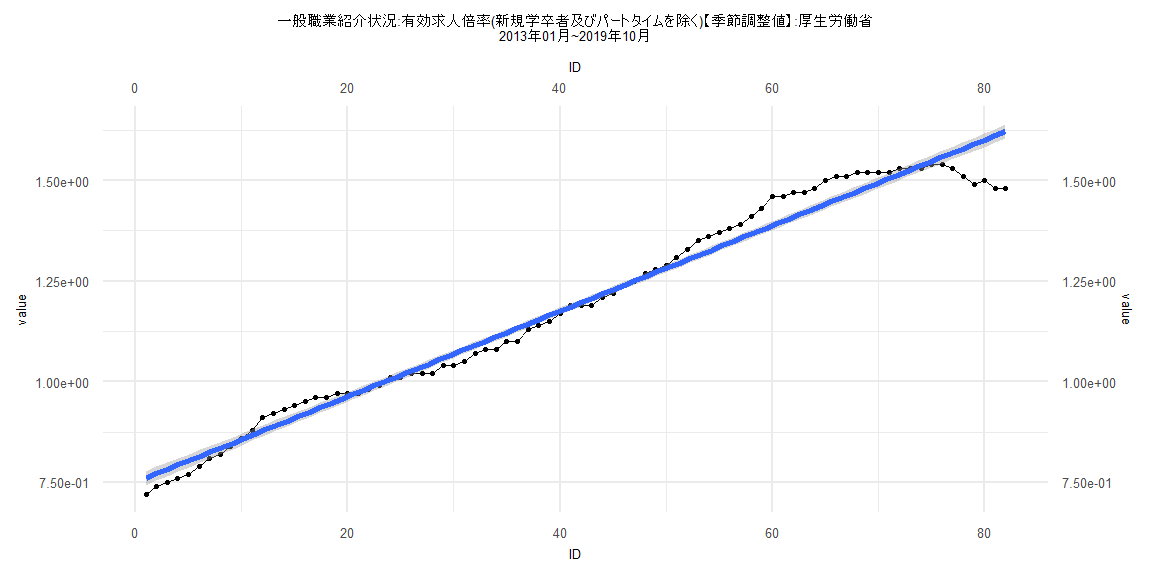
Call:
lm(formula = value ~ ID)

Residuals:
      Min        1Q    Median        3Q       Max
-0.139092 -0.019720 -0.000595  0.027047  0.072535

Coefficients:
             Estimate Std. Error t value            Pr(>|t|)
(Intercept) 0.7873418  0.0091436   86.11 <0.0000000000000002 ***
ID          0.0105285  0.0001986   53.02 <0.0000000000000002 ***
---
Signif. codes:  0 '***' 0.001 '**' 0.01 '*' 0.05 '.' 0.1 ' ' 1

Residual standard error: 0.04025 on 77 degrees of freedom
Multiple R-squared:  0.9733,    Adjusted R-squared:  0.973
F-statistic:  2811 on 1 and 77 DF,  p-value: < 0.00000000000000022


    Two-sample Kolmogorov-Smirnov test

data:  lm_residuals and rnorm(n = length(lm_residuals), mean = 0, sd = sd(lm_residuals))
D = 0.17722, p-value = 0.1677
alternative hypothesis: two-sided


    Durbin-Watson test

data:  value ~ ID
DW = 0.068021, p-value < 0.00000000000000022
alternative hypothesis: true autocorrelation is greater than 0


    studentized Breusch-Pagan test

data:  value ~ ID
BP = 17.918, df = 1, p-value = 0.00002307


    Box-Ljung test

data:  lm_residuals
X-squared = 63.921, df = 1, p-value = 0.000000000000001332