Analysis
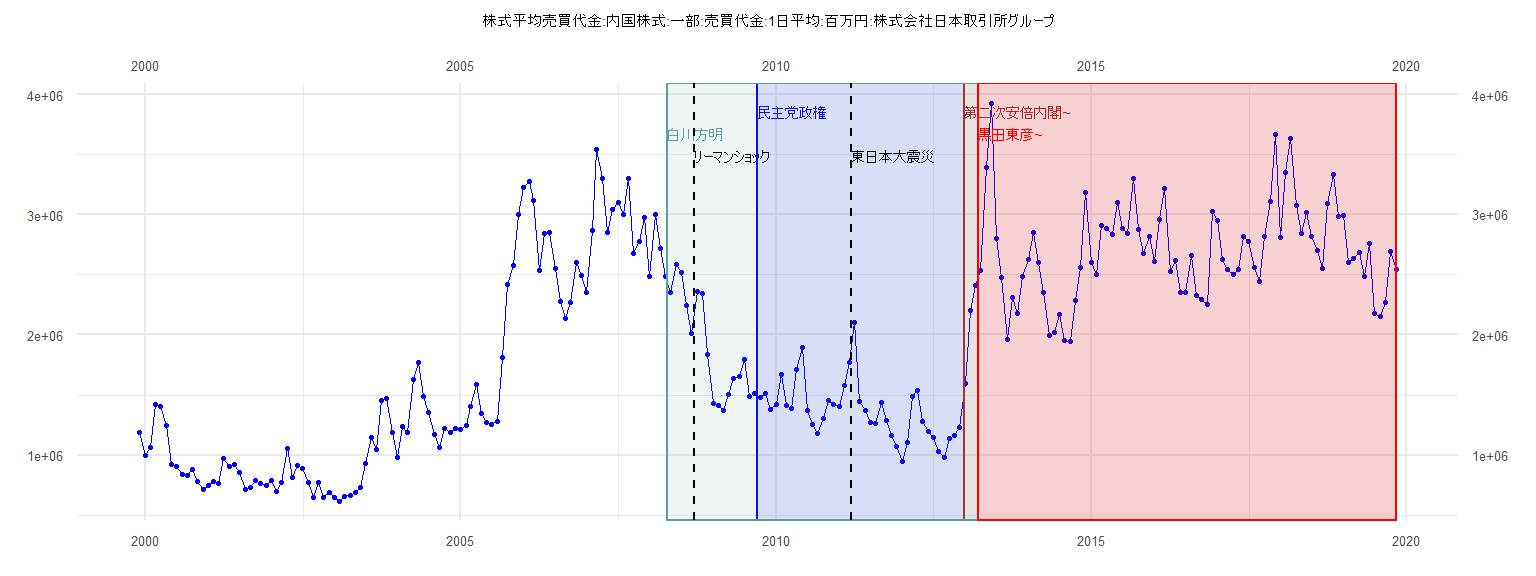
[1] "株式平均売買代金:内国株式:一部:売買代金:1日平均:百万円:株式会社日本取引所グループ"
         Jan     Feb     Mar     Apr     May     Jun     Jul     Aug     Sep     Oct     Nov     Dec
1999                                                                                 1190270  997131
2000 1065612 1423953 1401572 1242929  920692  907501  843227  830590  878884  780431  712746  744993
2001  783773  766107  974928  907208  926221  857046  713116  728824  792165  768405  746111  787767
2002  700687  770380 1058624  815055  911387  890467  770104  650081  776920  644281  692154  644484
2003  618597  659740  665502  691904  727446  932425 1149128 1048995 1456620 1474119 1187506  984390
2004 1242558 1192139 1628998 1772750 1486559 1358666 1176267 1066055 1218821 1191488 1220486 1216419
2005 1249814 1407819 1584125 1346660 1268646 1257471 1278306 1816680 2418753 2578389 3005621 3223037
2006 3272619 3117105 2533110 2846416 2848278 2550797 2278013 2135954 2269660 2600484 2497690 2352511
2007 2865176 3545261 3298899 2849570 3047014 3102085 3001339 3299086 2679483 2779445 2981175 2486611
2008 3004505 2716782 2484303 2351160 2585057 2516938 2241916 2010353 2358670 2348158 1838792 1429989
2009 1412669 1375946 1501132 1638853 1658454 1794484 1487329 1513037 1478630 1509394 1383657 1421421
2010 1670310 1409769 1391792 1709751 1894527 1370943 1255825 1177438 1306663 1452950 1418767 1402251
2011 1577937 1773305 2105237 1443220 1369539 1275402 1262152 1435452 1288385 1161690 1071715  950474
2012 1103033 1490064 1539904 1276379 1196318 1145316 1030783  978849 1136654 1164265 1226901 1593594
2013 2202269 2414066 2539406 3391862 3924916 2803719 2481552 1965620 2313087 2179362 2485873 2625938
2014 2852485 2601033 2356798 1997479 2022514 2168276 1952640 1947647 2287060 2557745 3182968 2603687
2015 2504939 2908712 2887224 2835424 3104931 2881951 2841807 3302245 2877702 2681361 2817305 2615000
2016 2961982 3222283 2526312 2616106 2354225 2351540 2664518 2331876 2298815 2255915 3023368 2950654
2017 2631057 2545715 2504086 2546934 2818867 2776371 2558166 2441106 2822167 3107697 3664844 2807537
2018 3350338 3631533 3075846 2843747 3021328 2820784 2701101 2556004 3092903 3332933 2981527 2990440
2019 2598955 2635621 2683901 2490223 2758853 2181869 2152049 2272770 2692279 2546099
Call:
lm(formula = value ~ ID)

Residuals:
    Min      1Q  Median      3Q     Max
-324723 -130491  -36877   76808  728375

Coefficients:
            Estimate Std. Error t value             Pr(>|t|)
(Intercept)  1591488      68557  23.214 < 0.0000000000000002 ***
ID            -11296       2987  -3.781             0.000552 ***
---
Signif. codes:  0 '***' 0.001 '**' 0.01 '*' 0.05 '.' 0.1 ' ' 1

Residual standard error: 210000 on 37 degrees of freedom
Multiple R-squared:  0.2787,    Adjusted R-squared:  0.2592
F-statistic:  14.3 on 1 and 37 DF,  p-value: 0.0005519


    Two-sample Kolmogorov-Smirnov test

data:  lm_residuals and rnorm(n = length(lm_residuals), mean = 0, sd = sd(lm_residuals))
D = 0.15385, p-value = 0.7523
alternative hypothesis: two-sided


    Durbin-Watson test

data:  value ~ ID
DW = 1.004, p-value = 0.0001947
alternative hypothesis: true autocorrelation is greater than 0


    studentized Breusch-Pagan test

data:  value ~ ID
BP = 0.079428, df = 1, p-value = 0.7781


    Box-Ljung test

data:  lm_residuals
X-squared = 10.23, df = 1, p-value = 0.001381
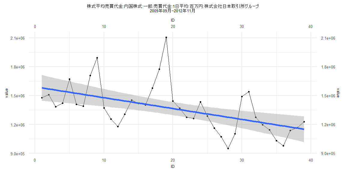
Call:
lm(formula = value ~ ID)

Residuals:
    Min      1Q  Median      3Q     Max
-919302 -261574  -41348  250603 1392430

Coefficients:
            Estimate Std. Error t value            Pr(>|t|)
(Intercept)  2508978      89768   27.95 <0.0000000000000002 ***
ID              3918       1856    2.11              0.0379 *
---
Signif. codes:  0 '***' 0.001 '**' 0.01 '*' 0.05 '.' 0.1 ' ' 1

Residual standard error: 405200 on 81 degrees of freedom
Multiple R-squared:  0.05212,   Adjusted R-squared:  0.04042
F-statistic: 4.454 on 1 and 81 DF,  p-value: 0.03791


    Two-sample Kolmogorov-Smirnov test

data:  lm_residuals and rnorm(n = length(lm_residuals), mean = 0, sd = sd(lm_residuals))
D = 0.096386, p-value = 0.8386
alternative hypothesis: two-sided


    Durbin-Watson test

data:  value ~ ID
DW = 0.79652, p-value = 0.0000000002024
alternative hypothesis: true autocorrelation is greater than 0


    studentized Breusch-Pagan test

data:  value ~ ID
BP = 2.6313, df = 1, p-value = 0.1048


    Box-Ljung test

data:  lm_residuals
X-squared = 27.645, df = 1, p-value = 0.0000001457
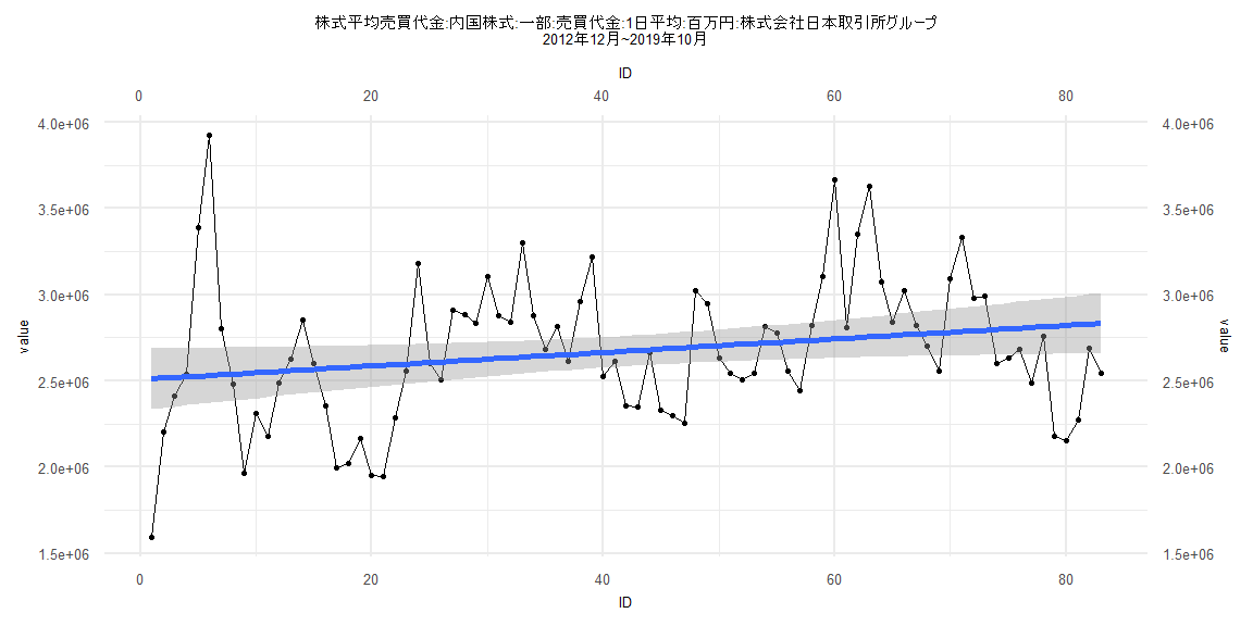
Call:
lm(formula = value ~ ID)

Residuals:
    Min      1Q  Median      3Q     Max
-417044 -234352 -109920  122088 1218130

Coefficients:
            Estimate Std. Error t value             Pr(>|t|)
(Intercept)  1919029      92787  20.682 < 0.0000000000000002 ***
ID            -12256       2690  -4.556            0.0000279 ***
---
Signif. codes:  0 '***' 0.001 '**' 0.01 '*' 0.05 '.' 0.1 ' ' 1

Residual standard error: 351800 on 57 degrees of freedom
Multiple R-squared:  0.267, Adjusted R-squared:  0.2541
F-statistic: 20.76 on 1 and 57 DF,  p-value: 0.00002794


    Two-sample Kolmogorov-Smirnov test

data:  lm_residuals and rnorm(n = length(lm_residuals), mean = 0, sd = sd(lm_residuals))
D = 0.28814, p-value = 0.01452
alternative hypothesis: two-sided


    Durbin-Watson test

data:  value ~ ID
DW = 0.43744, p-value = 0.000000000000009077
alternative hypothesis: true autocorrelation is greater than 0


    studentized Breusch-Pagan test

data:  value ~ ID
BP = 0.75132, df = 1, p-value = 0.3861


    Box-Ljung test

data:  lm_residuals
X-squared = 27.205, df = 1, p-value = 0.000000183
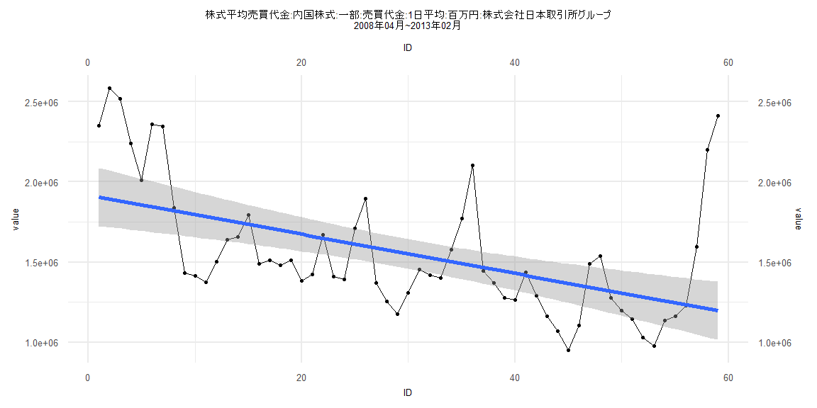
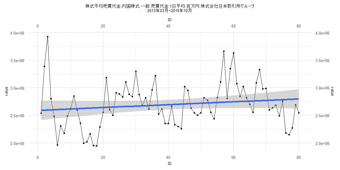
Call:
lm(formula = value ~ ID)

Residuals:
    Min      1Q  Median      3Q     Max
-690136 -256430  -49369  221483 1326057

Coefficients:
            Estimate Std. Error t value            Pr(>|t|)
(Intercept)  2591074      89445  28.968 <0.0000000000000002 ***
ID              2595       1919   1.353                0.18
---
Signif. codes:  0 '***' 0.001 '**' 0.01 '*' 0.05 '.' 0.1 ' ' 1

Residual standard error: 396300 on 78 degrees of freedom
Multiple R-squared:  0.02292,   Adjusted R-squared:  0.01039
F-statistic: 1.829 on 1 and 78 DF,  p-value: 0.1801


    Two-sample Kolmogorov-Smirnov test

data:  lm_residuals and rnorm(n = length(lm_residuals), mean = 0, sd = sd(lm_residuals))
D = 0.15, p-value = 0.3307
alternative hypothesis: two-sided


    Durbin-Watson test

data:  value ~ ID
DW = 0.83032, p-value = 0.000000001494
alternative hypothesis: true autocorrelation is greater than 0


    studentized Breusch-Pagan test

data:  value ~ ID
BP = 2.2984, df = 1, p-value = 0.1295


    Box-Ljung test

data:  lm_residuals
X-squared = 28.138, df = 1, p-value = 0.000000113