Analysis
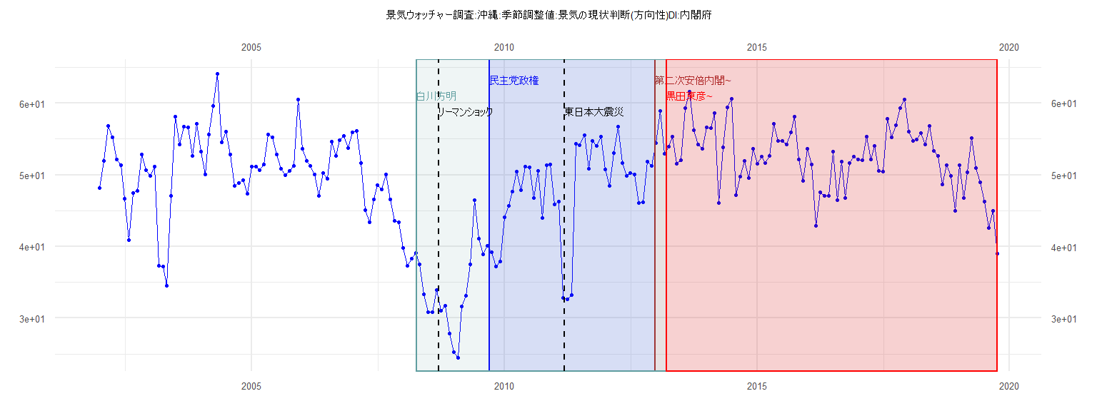
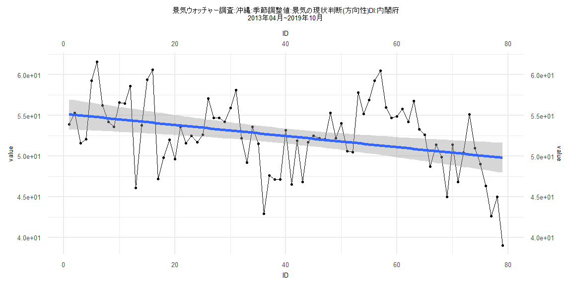
[1] "景気ウォッチャー調査:沖縄:季節調整値:景気の現状判断(方向性)DI:内閣府"
      Jan  Feb  Mar  Apr  May  Jun  Jul  Aug  Sep  Oct  Nov  Dec
2002 48.2 52.0 56.8 55.2 52.2 51.4 46.7 40.9 47.5 47.8 52.8 50.7
2003 49.9 51.2 37.3 37.2 34.5 47.1 58.1 54.2 56.7 56.6 52.6 57.1
2004 53.2 50.1 55.6 59.6 64.1 54.5 56.0 52.8 48.5 48.9 49.3 47.4
2005 51.2 51.2 50.7 51.5 55.6 55.2 52.8 50.9 50.0 50.6 51.3 60.5
2006 53.6 52.0 51.3 50.1 47.1 50.3 49.5 54.6 52.6 54.8 55.4 53.7
2007 55.9 56.1 51.7 45.1 43.4 46.6 48.6 48.0 50.1 46.6 43.6 43.4
2008 39.8 37.3 38.3 39.1 37.5 33.3 30.8 30.8 33.9 31.0 31.7 27.8
2009 25.3 24.5 31.6 33.1 37.5 46.5 41.1 38.9 40.1 39.2 37.2 37.9
2010 44.1 45.7 47.7 50.5 47.9 51.2 51.1 46.8 50.6 44.0 51.4 51.5
2011 45.9 46.3 32.8 32.6 33.2 54.3 54.1 55.5 50.9 54.7 54.0 55.3
2012 50.8 48.5 53.0 56.7 51.7 49.9 50.3 50.1 46.1 46.2 51.9 51.3
2013 54.4 58.9 52.9 53.9 55.3 51.6 52.1 59.3 61.6 56.2 54.2 53.6
2014 56.6 56.5 58.6 46.1 53.8 59.4 60.6 47.2 49.8 52.0 49.6 53.6
2015 51.6 52.5 51.7 52.6 57.1 54.7 54.7 54.2 55.9 58.1 52.2 49.2
2016 53.6 51.5 42.9 47.6 47.1 47.1 53.2 46.5 51.9 46.8 51.7 52.5
2017 52.2 52.1 55.3 52.2 54.0 50.6 50.5 57.8 55.2 56.9 59.3 60.5
2018 56.0 54.7 54.9 55.8 54.2 56.8 53.3 52.6 48.7 51.4 49.9 45.0
2019 51.4 46.8 50.4 55.1 51.0 49.0 46.3 42.6 45.0 39.0
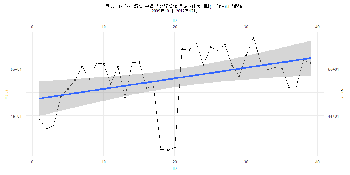
Call:
lm(formula = value ~ ID)

Residuals:
     Min       1Q   Median       3Q      Max
-15.1950  -1.4602   0.9398   4.6815   6.7926

Coefficients:
            Estimate Std. Error t value             Pr(>|t|)
(Intercept) 43.46113    1.91504  22.695 < 0.0000000000000002 ***
ID           0.22810    0.08345   2.733              0.00956 **
---
Signif. codes:  0 '***' 0.001 '**' 0.01 '*' 0.05 '.' 0.1 ' ' 1

Residual standard error: 5.865 on 37 degrees of freedom
Multiple R-squared:  0.168, Adjusted R-squared:  0.1455
F-statistic: 7.472 on 1 and 37 DF,  p-value: 0.009557


    Two-sample Kolmogorov-Smirnov test

data:  lm_residuals and rnorm(n = length(lm_residuals), mean = 0, sd = sd(lm_residuals))
D = 0.12821, p-value = 0.9114
alternative hypothesis: two-sided


    Durbin-Watson test

data:  value ~ ID
DW = 0.81605, p-value = 0.00000751
alternative hypothesis: true autocorrelation is greater than 0


    studentized Breusch-Pagan test

data:  value ~ ID
BP = 0.20385, df = 1, p-value = 0.6516


    Box-Ljung test

data:  lm_residuals
X-squared = 14.332, df = 1, p-value = 0.0001532
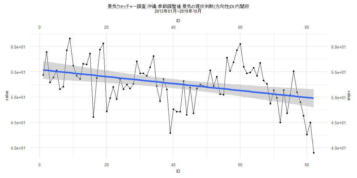
Call:
lm(formula = value ~ ID)

Residuals:
     Min       1Q   Median       3Q      Max
-10.7899  -2.0789   0.1188   3.1155   9.1969

Coefficients:
            Estimate Std. Error t value             Pr(>|t|)
(Intercept) 55.43008    0.91334  60.689 < 0.0000000000000002 ***
ID          -0.06878    0.01912  -3.598             0.000554 ***
---
Signif. codes:  0 '***' 0.001 '**' 0.01 '*' 0.05 '.' 0.1 ' ' 1

Residual standard error: 4.098 on 80 degrees of freedom
Multiple R-squared:  0.1393,    Adjusted R-squared:  0.1285
F-statistic: 12.94 on 1 and 80 DF,  p-value: 0.000554


    Two-sample Kolmogorov-Smirnov test

data:  lm_residuals and rnorm(n = length(lm_residuals), mean = 0, sd = sd(lm_residuals))
D = 0.073171, p-value = 0.9818
alternative hypothesis: two-sided


    Durbin-Watson test

data:  value ~ ID
DW = 1.0289, p-value = 0.0000006773
alternative hypothesis: true autocorrelation is greater than 0


    studentized Breusch-Pagan test

data:  value ~ ID
BP = 2.2675, df = 1, p-value = 0.1321


    Box-Ljung test

data:  lm_residuals
X-squared = 16.603, df = 1, p-value = 0.00004607
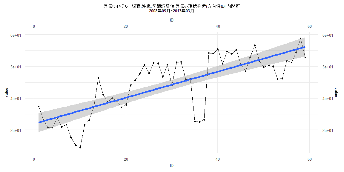
Call:
lm(formula = value ~ ID)

Residuals:
     Min       1Q   Median       3Q      Max
-14.1764  -3.0068   0.3293   5.0441   8.7541

Coefficients:
            Estimate Std. Error t value             Pr(>|t|)
(Intercept) 31.99918    1.55129  20.627 < 0.0000000000000002 ***
ID           0.41048    0.04497   9.128    0.000000000000955 ***
---
Signif. codes:  0 '***' 0.001 '**' 0.01 '*' 0.05 '.' 0.1 ' ' 1

Residual standard error: 5.882 on 57 degrees of freedom
Multiple R-squared:  0.5938,    Adjusted R-squared:  0.5867
F-statistic: 83.32 on 1 and 57 DF,  p-value: 0.0000000000009551


    Two-sample Kolmogorov-Smirnov test

data:  lm_residuals and rnorm(n = length(lm_residuals), mean = 0, sd = sd(lm_residuals))
D = 0.13559, p-value = 0.6544
alternative hypothesis: two-sided


    Durbin-Watson test

data:  value ~ ID
DW = 0.68903, p-value = 0.000000001441
alternative hypothesis: true autocorrelation is greater than 0


    studentized Breusch-Pagan test

data:  value ~ ID
BP = 0.017378, df = 1, p-value = 0.8951


    Box-Ljung test

data:  lm_residuals
X-squared = 25.905, df = 1, p-value = 0.0000003586
Call:
lm(formula = value ~ ID)

Residuals:
     Min       1Q   Median       3Q      Max
-10.7997  -2.0446   0.1213   2.9922   9.1949

Coefficients:
            Estimate Std. Error t value             Pr(>|t|)
(Intercept) 55.20545    0.94195  58.608 < 0.0000000000000002 ***
ID          -0.06843    0.02046  -3.345              0.00127 **
---
Signif. codes:  0 '***' 0.001 '**' 0.01 '*' 0.05 '.' 0.1 ' ' 1

Residual standard error: 4.146 on 77 degrees of freedom
Multiple R-squared:  0.1269,    Adjusted R-squared:  0.1155
F-statistic: 11.19 on 1 and 77 DF,  p-value: 0.001274


    Two-sample Kolmogorov-Smirnov test

data:  lm_residuals and rnorm(n = length(lm_residuals), mean = 0, sd = sd(lm_residuals))
D = 0.10127, p-value = 0.8161
alternative hypothesis: two-sided


    Durbin-Watson test

data:  value ~ ID
DW = 1.0007, p-value = 0.0000004716
alternative hypothesis: true autocorrelation is greater than 0


    studentized Breusch-Pagan test

data:  value ~ ID
BP = 1.7112, df = 1, p-value = 0.1908


    Box-Ljung test

data:  lm_residuals
X-squared = 16.984, df = 1, p-value = 0.00003769