Analysis
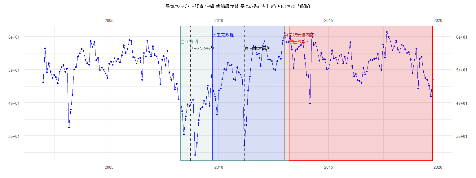
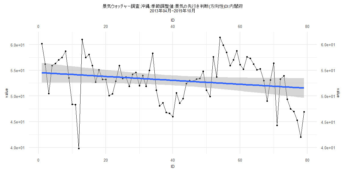
[1] "景気ウォッチャー調査:沖縄:季節調整値:景気の先行き判断(方向性)DI:内閣府"
      Jan  Feb  Mar  Apr  May  Jun  Jul  Aug  Sep  Oct  Nov  Dec
2002 46.2 56.5 49.3 52.0 49.4 47.5 48.4 47.8 45.8 49.5 50.8 51.4
2003 49.4 50.4 32.6 38.0 42.4 50.1 50.9 53.9 55.0 56.3 55.7 53.0
2004 52.0 51.5 58.7 56.9 58.4 52.9 53.6 49.9 50.7 50.0 48.9 47.5
2005 51.8 52.4 51.5 53.5 52.5 53.4 52.3 54.4 57.4 55.1 56.3 59.0
2006 58.7 53.8 53.7 51.9 53.4 53.6 46.9 55.1 54.0 58.8 55.4 54.0
2007 57.1 54.3 54.0 52.4 45.5 53.0 54.1 51.2 55.8 49.2 46.9 48.7
2008 44.1 45.8 41.1 40.8 37.5 30.5 35.9 39.6 39.0 40.1 41.0 24.3
2009 27.9 34.8 38.2 38.6 40.6 39.7 45.3 39.1 48.3 43.6 41.9 36.5
2010 43.8 44.3 47.1 50.2 49.9 52.1 51.3 51.5 47.1 46.9 50.8 49.2
2011 48.5 47.0 27.1 33.3 43.7 48.0 53.1 57.2 56.1 54.6 54.9 51.1
2012 57.3 58.6 56.1 53.1 53.0 52.6 50.3 49.9 52.5 54.0 53.3 58.8
2013 61.1 58.4 58.3 60.2 56.2 50.5 55.9 56.3 57.0 57.5 58.7 53.5
2014 48.4 48.3 39.8 61.0 57.5 58.1 55.9 52.7 55.1 53.2 53.2 50.1
2015 50.4 52.9 55.9 53.4 53.7 51.9 54.2 54.6 52.0 54.0 51.9 55.0
2016 58.3 51.1 48.1 48.7 46.8 46.6 46.0 50.6 48.6 49.5 52.4 53.0
2017 52.9 53.3 53.4 54.8 51.1 49.9 57.6 53.7 61.4 59.9 58.5 55.9
2018 57.0 58.8 56.1 55.2 57.6 57.3 56.2 55.1 55.3 53.0 49.0 53.1
2019 56.4 44.3 53.3 53.9 49.4 47.5 47.0 45.3 42.0 46.9
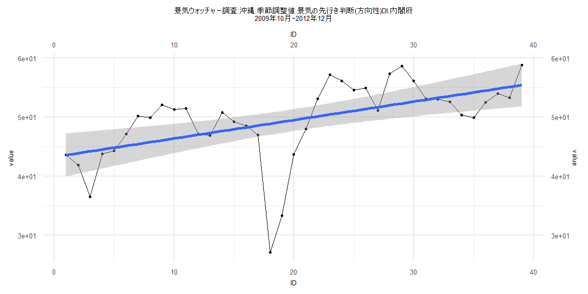
Call:
lm(formula = value ~ ID)

Residuals:
     Min       1Q   Median       3Q      Max
-21.7709  -1.6829   0.1008   3.5393   6.7692

Coefficients:
            Estimate Std. Error t value             Pr(>|t|)
(Intercept) 43.25560    1.86640  23.176 < 0.0000000000000002 ***
ID           0.31196    0.08133   3.836             0.000471 ***
---
Signif. codes:  0 '***' 0.001 '**' 0.01 '*' 0.05 '.' 0.1 ' ' 1

Residual standard error: 5.716 on 37 degrees of freedom
Multiple R-squared:  0.2845,    Adjusted R-squared:  0.2652
F-statistic: 14.71 on 1 and 37 DF,  p-value: 0.0004712


    Two-sample Kolmogorov-Smirnov test

data:  lm_residuals and rnorm(n = length(lm_residuals), mean = 0, sd = sd(lm_residuals))
D = 0.30769, p-value = 0.04927
alternative hypothesis: two-sided


    Durbin-Watson test

data:  value ~ ID
DW = 0.71587, p-value = 0.0000008423
alternative hypothesis: true autocorrelation is greater than 0


    studentized Breusch-Pagan test

data:  value ~ ID
BP = 0.10092, df = 1, p-value = 0.7507


    Box-Ljung test

data:  lm_residuals
X-squared = 17.093, df = 1, p-value = 0.00003559
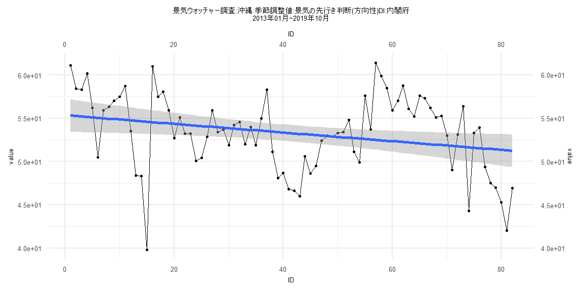
Call:
lm(formula = value ~ ID)

Residuals:
    Min      1Q  Median      3Q     Max
-14.803  -2.700   0.525   3.134   8.900

Coefficients:
            Estimate Std. Error t value            Pr(>|t|)
(Intercept) 55.35357    0.96375  57.436 <0.0000000000000002 ***
ID          -0.05007    0.02017  -2.482              0.0152 *
---
Signif. codes:  0 '***' 0.001 '**' 0.01 '*' 0.05 '.' 0.1 ' ' 1

Residual standard error: 4.324 on 80 degrees of freedom
Multiple R-squared:  0.07151,   Adjusted R-squared:  0.0599
F-statistic: 6.161 on 1 and 80 DF,  p-value: 0.01515


    Two-sample Kolmogorov-Smirnov test

data:  lm_residuals and rnorm(n = length(lm_residuals), mean = 0, sd = sd(lm_residuals))
D = 0.15854, p-value = 0.2552
alternative hypothesis: two-sided


    Durbin-Watson test

data:  value ~ ID
DW = 0.9352, p-value = 0.00000003999
alternative hypothesis: true autocorrelation is greater than 0


    studentized Breusch-Pagan test

data:  value ~ ID
BP = 0.17861, df = 1, p-value = 0.6726


    Box-Ljung test

data:  lm_residuals
X-squared = 22.541, df = 1, p-value = 0.000002058
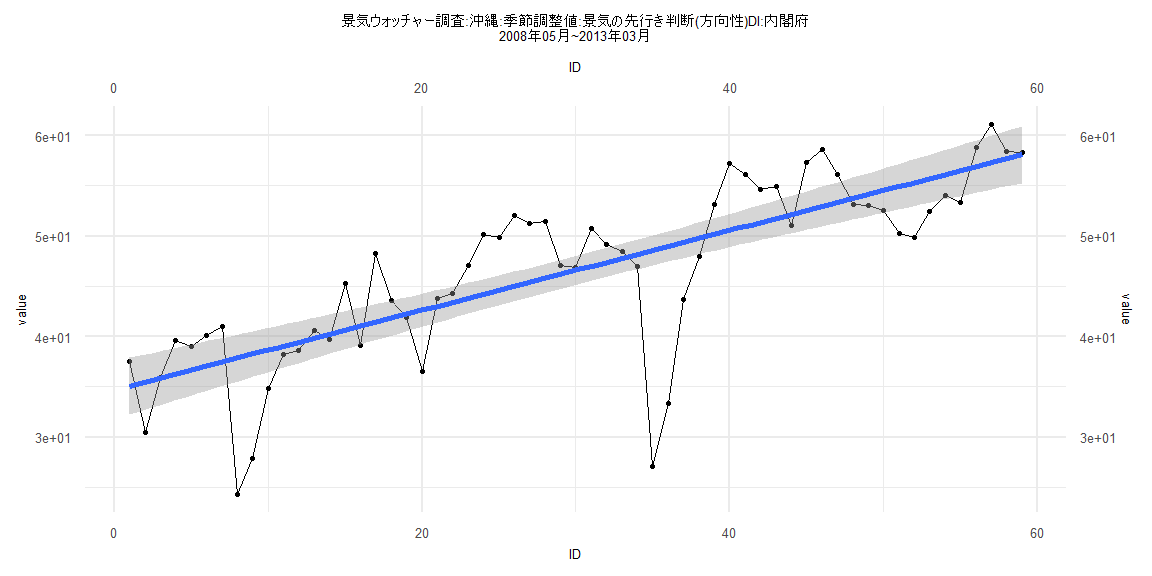
Call:
lm(formula = value ~ ID)

Residuals:
     Min       1Q   Median       3Q      Max
-21.4692  -1.8411   0.7623   3.3139   7.1028

Coefficients:
            Estimate Std. Error t value             Pr(>|t|)
(Intercept) 34.67820    1.44442  24.008 < 0.0000000000000002 ***
ID           0.39688    0.04187   9.479    0.000000000000258 ***
---
Signif. codes:  0 '***' 0.001 '**' 0.01 '*' 0.05 '.' 0.1 ' ' 1

Residual standard error: 5.477 on 57 degrees of freedom
Multiple R-squared:  0.6118,    Adjusted R-squared:  0.605
F-statistic: 89.84 on 1 and 57 DF,  p-value: 0.0000000000002578


    Two-sample Kolmogorov-Smirnov test

data:  lm_residuals and rnorm(n = length(lm_residuals), mean = 0, sd = sd(lm_residuals))
D = 0.13559, p-value = 0.6544
alternative hypothesis: two-sided


    Durbin-Watson test

data:  value ~ ID
DW = 0.87912, p-value = 0.0000005104
alternative hypothesis: true autocorrelation is greater than 0


    studentized Breusch-Pagan test

data:  value ~ ID
BP = 0.059449, df = 1, p-value = 0.8074


    Box-Ljung test

data:  lm_residuals
X-squared = 19.37, df = 1, p-value = 0.00001077
Call:
lm(formula = value ~ ID)

Residuals:
    Min      1Q  Median      3Q     Max
-14.312  -2.857   0.610   3.100   8.884

Coefficients:
            Estimate Std. Error t value            Pr(>|t|)
(Intercept) 54.56767    0.98057  55.649 <0.0000000000000002 ***
ID          -0.03799    0.02130  -1.784              0.0784 .
---
Signif. codes:  0 '***' 0.001 '**' 0.01 '*' 0.05 '.' 0.1 ' ' 1

Residual standard error: 4.316 on 77 degrees of freedom
Multiple R-squared:  0.03968,   Adjusted R-squared:  0.02721
F-statistic: 3.182 on 1 and 77 DF,  p-value: 0.07839


    Two-sample Kolmogorov-Smirnov test

data:  lm_residuals and rnorm(n = length(lm_residuals), mean = 0, sd = sd(lm_residuals))
D = 0.1519, p-value = 0.3233
alternative hypothesis: two-sided


    Durbin-Watson test

data:  value ~ ID
DW = 0.96753, p-value = 0.0000001798
alternative hypothesis: true autocorrelation is greater than 0


    studentized Breusch-Pagan test

data:  value ~ ID
BP = 0.27545, df = 1, p-value = 0.5997


    Box-Ljung test

data:  lm_residuals
X-squared = 20.3, df = 1, p-value = 0.00000662