Analysis
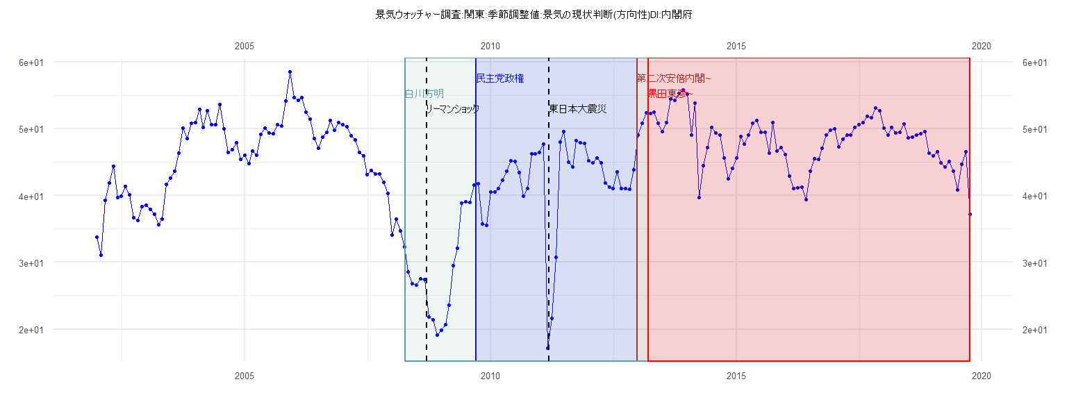
[1] "景気ウォッチャー調査:関東:季節調整値:景気の現状判断(方向性)DI:内閣府"
      Jan  Feb  Mar  Apr  May  Jun  Jul  Aug  Sep  Oct  Nov  Dec
2002 33.8 31.1 39.3 41.9 44.4 39.7 39.9 41.4 40.1 36.7 36.3 38.3
2003 38.6 37.9 37.2 35.6 36.5 41.7 42.6 43.7 46.3 50.1 48.5 50.8
2004 50.9 52.9 50.2 52.7 50.6 50.6 53.6 50.0 46.5 46.9 47.9 45.4
2005 46.0 44.8 46.7 46.0 49.2 50.1 49.4 49.3 50.6 50.4 54.1 58.5
2006 54.7 54.2 54.7 52.5 51.4 48.5 47.1 48.7 49.5 51.2 49.8 50.9
2007 50.6 50.3 48.9 48.3 46.5 45.9 43.1 43.8 43.2 43.2 42.0 40.3
2008 34.1 36.5 34.7 32.3 28.6 26.8 26.6 27.5 27.4 21.8 21.4 19.1
2009 19.9 20.7 23.6 29.5 32.1 38.9 39.1 39.0 41.6 41.8 35.8 35.5
2010 40.5 40.5 41.1 42.3 43.7 45.2 45.1 43.4 39.9 41.0 46.2 46.2
2011 46.5 47.7 17.2 21.6 30.8 48.0 49.6 45.0 44.3 48.2 47.9 47.8
2012 45.2 44.9 45.6 44.9 41.9 41.3 41.1 43.5 41.1 41.1 40.9 43.9
2013 49.1 50.8 52.4 52.3 52.5 50.8 49.6 50.9 54.5 54.2 55.3 55.8
2014 55.2 49.1 53.8 39.7 44.5 47.2 50.2 49.4 49.1 45.6 42.5 44.1
2015 45.6 48.8 47.7 49.1 50.8 51.2 49.5 49.5 46.3 50.9 46.7 47.2
2016 46.1 42.9 41.0 41.2 41.3 39.4 43.6 45.5 45.4 47.1 49.0 49.8
2017 50.0 47.3 48.4 49.1 49.1 50.2 50.6 50.9 51.9 51.6 53.1 52.7
2018 50.1 49.1 50.2 49.4 49.5 50.7 48.6 48.7 49.0 49.3 49.6 46.3
2019 45.9 46.6 44.9 44.3 45.1 43.6 40.8 44.7 46.6 37.2
Call:
lm(formula = value ~ ID)

Residuals:
    Min      1Q  Median      3Q     Max
-24.624  -1.631   1.513   4.094   7.414

Coefficients:
            Estimate Std. Error t value            Pr(>|t|)
(Intercept) 40.19703    2.13739  18.807 <0.0000000000000002 ***
ID           0.09040    0.09314   0.971               0.338
---
Signif. codes:  0 '***' 0.001 '**' 0.01 '*' 0.05 '.' 0.1 ' ' 1

Residual standard error: 6.546 on 37 degrees of freedom
Multiple R-squared:  0.02483,   Adjusted R-squared:  -0.001523
F-statistic: 0.9422 on 1 and 37 DF,  p-value: 0.338


    Two-sample Kolmogorov-Smirnov test

data:  lm_residuals and rnorm(n = length(lm_residuals), mean = 0, sd = sd(lm_residuals))
D = 0.38462, p-value = 0.00581
alternative hypothesis: two-sided


    Durbin-Watson test

data:  value ~ ID
DW = 0.95829, p-value = 0.00009605
alternative hypothesis: true autocorrelation is greater than 0


    studentized Breusch-Pagan test

data:  value ~ ID
BP = 0.068584, df = 1, p-value = 0.7934


    Box-Ljung test

data:  lm_residuals
X-squared = 11.383, df = 1, p-value = 0.000741
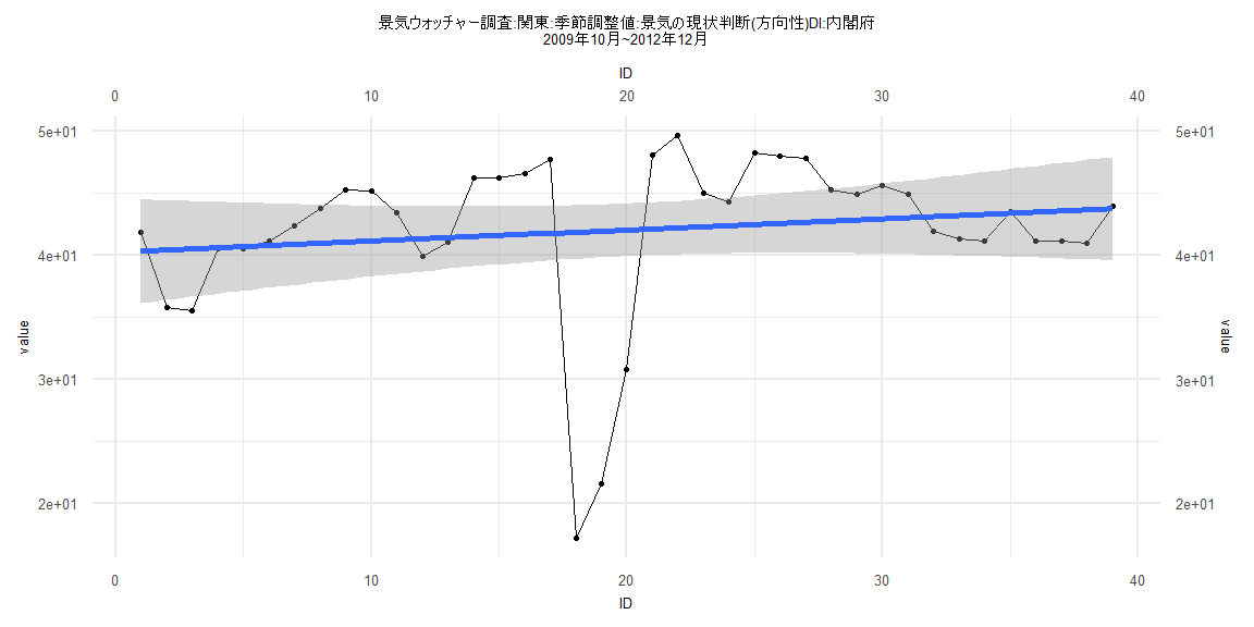
Call:
lm(formula = value ~ ID)

Residuals:
    Min      1Q  Median      3Q     Max
-9.8365 -1.9553  0.6456  2.4062  6.0480

Coefficients:
            Estimate Std. Error t value             Pr(>|t|)
(Intercept) 50.39874    0.81556  61.796 < 0.0000000000000002 ***
ID          -0.05389    0.01707  -3.157              0.00225 **
---
Signif. codes:  0 '***' 0.001 '**' 0.01 '*' 0.05 '.' 0.1 ' ' 1

Residual standard error: 3.659 on 80 degrees of freedom
Multiple R-squared:  0.1108,    Adjusted R-squared:  0.09967
F-statistic: 9.967 on 1 and 80 DF,  p-value: 0.002248


    Two-sample Kolmogorov-Smirnov test

data:  lm_residuals and rnorm(n = length(lm_residuals), mean = 0, sd = sd(lm_residuals))
D = 0.097561, p-value = 0.8332
alternative hypothesis: two-sided


    Durbin-Watson test

data:  value ~ ID
DW = 0.58672, p-value = 0.00000000000000751
alternative hypothesis: true autocorrelation is greater than 0


    studentized Breusch-Pagan test

data:  value ~ ID
BP = 0.16811, df = 1, p-value = 0.6818


    Box-Ljung test

data:  lm_residuals
X-squared = 38.165, df = 1, p-value = 0.00000000065
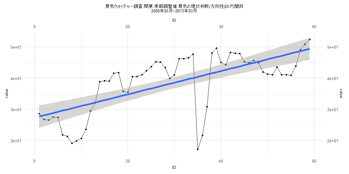
Call:
lm(formula = value ~ ID)

Residuals:
    Min      1Q  Median      3Q     Max
-23.213  -4.054   1.049   5.646   8.151

Coefficients:
            Estimate Std. Error t value             Pr(>|t|)
(Intercept) 27.33063    1.83406   14.90 < 0.0000000000000002 ***
ID           0.37378    0.05317    7.03        0.00000000283 ***
---
Signif. codes:  0 '***' 0.001 '**' 0.01 '*' 0.05 '.' 0.1 ' ' 1

Residual standard error: 6.954 on 57 degrees of freedom
Multiple R-squared:  0.4644,    Adjusted R-squared:  0.455
F-statistic: 49.43 on 1 and 57 DF,  p-value: 0.000000002832


    Two-sample Kolmogorov-Smirnov test

data:  lm_residuals and rnorm(n = length(lm_residuals), mean = 0, sd = sd(lm_residuals))
D = 0.25424, p-value = 0.04374
alternative hypothesis: two-sided


    Durbin-Watson test

data:  value ~ ID
DW = 0.61212, p-value = 0.00000000007104
alternative hypothesis: true autocorrelation is greater than 0


    studentized Breusch-Pagan test

data:  value ~ ID
BP = 0.099684, df = 1, p-value = 0.7522


    Box-Ljung test

data:  lm_residuals
X-squared = 29.727, df = 1, p-value = 0.00000004974
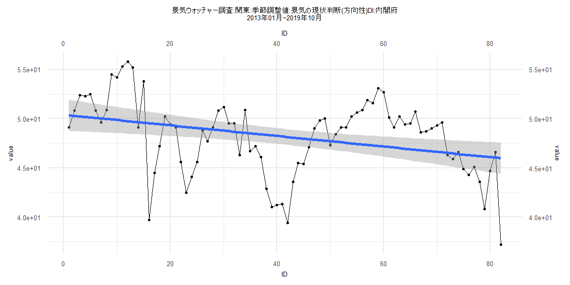
Call:
lm(formula = value ~ ID)

Residuals:
    Min      1Q  Median      3Q     Max
-9.7822 -2.1031  0.7571  2.4469  6.1076

Coefficients:
            Estimate Std. Error t value             Pr(>|t|)
(Intercept) 50.16534    0.84462  59.394 < 0.0000000000000002 ***
ID          -0.05255    0.01834  -2.865              0.00538 **
---
Signif. codes:  0 '***' 0.001 '**' 0.01 '*' 0.05 '.' 0.1 ' ' 1

Residual standard error: 3.718 on 77 degrees of freedom
Multiple R-squared:  0.09632,   Adjusted R-squared:  0.08458
F-statistic: 8.207 on 1 and 77 DF,  p-value: 0.005377


    Two-sample Kolmogorov-Smirnov test

data:  lm_residuals and rnorm(n = length(lm_residuals), mean = 0, sd = sd(lm_residuals))
D = 0.13924, p-value = 0.4302
alternative hypothesis: two-sided


    Durbin-Watson test

data:  value ~ ID
DW = 0.58492, p-value = 0.00000000000001932
alternative hypothesis: true autocorrelation is greater than 0


    studentized Breusch-Pagan test

data:  value ~ ID
BP = 0.6196, df = 1, p-value = 0.4312


    Box-Ljung test

data:  lm_residuals
X-squared = 36.695, df = 1, p-value = 0.000000001381