Analysis
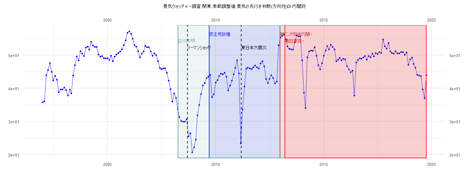
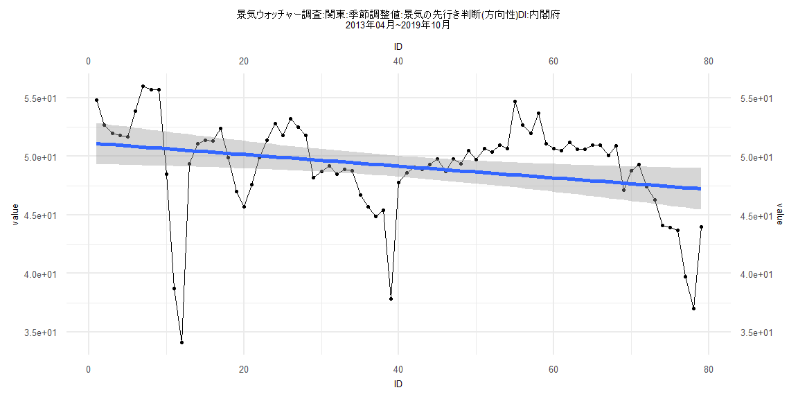
[1] "景気ウォッチャー調査:関東:季節調整値:景気の先行き判断(方向性)DI:内閣府"
      Jan  Feb  Mar  Apr  May  Jun  Jul  Aug  Sep  Oct  Nov  Dec
2002 35.8 36.1 44.0 45.5 47.7 45.0 42.4 43.8 42.6 38.8 39.7 39.7
2003 40.2 39.5 37.8 39.6 38.5 43.9 47.0 49.7 48.5 51.2 50.5 49.8
2004 52.3 52.6 51.7 54.1 53.0 52.5 52.5 50.2 49.6 49.8 49.1 49.0
2005 49.1 48.6 49.9 48.2 49.6 50.2 50.7 51.1 51.8 53.1 54.5 56.8
2006 57.2 56.5 55.0 53.1 52.6 51.2 49.4 50.5 51.1 52.9 52.4 52.4
2007 51.1 49.9 50.6 50.0 48.2 46.2 45.8 46.0 46.1 44.7 42.3 39.8
2008 36.0 38.5 37.1 33.6 31.3 30.1 29.9 29.9 30.7 25.5 26.4 20.7
2009 22.1 24.5 31.9 35.0 38.3 40.9 41.6 43.2 43.5 44.1 37.4 38.2
2010 41.8 42.5 43.7 44.4 44.3 44.7 43.5 39.4 40.9 42.3 44.3 46.2
2011 48.5 44.5 23.3 33.6 40.6 45.9 46.3 46.0 45.8 46.4 46.9 46.4
2012 46.0 47.6 48.2 46.6 42.8 41.6 42.9 44.0 43.2 41.5 42.1 53.0
2013 55.4 55.8 56.4 54.8 52.7 52.0 51.8 51.7 53.9 56.0 55.7 55.7
2014 48.5 38.7 34.1 49.4 51.1 51.4 51.3 52.4 49.9 47.0 45.7 47.6
2015 49.9 51.4 52.8 51.8 53.2 52.5 51.8 48.2 48.7 49.2 48.5 48.9
2016 48.8 46.7 45.7 44.9 45.4 37.8 47.8 48.6 49.1 48.9 49.3 49.8
2017 48.7 49.8 49.4 50.5 49.7 50.7 50.4 51.0 50.7 54.7 52.7 52.0
2018 53.7 51.1 50.7 50.5 51.2 50.6 50.6 51.0 51.0 50.1 50.9 47.1
2019 48.8 49.3 47.4 46.3 44.1 43.9 43.7 39.7 37.0 44.0
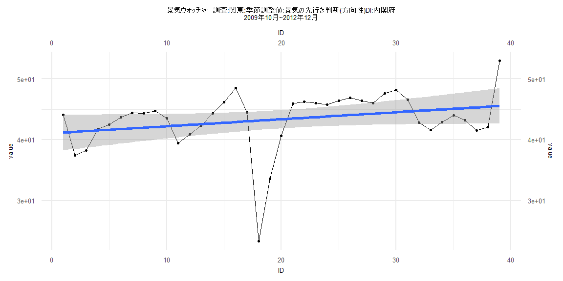
Call:
lm(formula = value ~ ID)

Residuals:
    Min      1Q  Median      3Q     Max
-19.839  -2.047   1.622   2.491   7.443

Coefficients:
            Estimate Std. Error t value            Pr(>|t|)
(Intercept)  41.0660     1.5078  27.236 <0.0000000000000002 ***
ID            0.1152     0.0657   1.753              0.0879 .
---
Signif. codes:  0 '***' 0.001 '**' 0.01 '*' 0.05 '.' 0.1 ' ' 1

Residual standard error: 4.618 on 37 degrees of freedom
Multiple R-squared:  0.07667,   Adjusted R-squared:  0.05172
F-statistic: 3.072 on 1 and 37 DF,  p-value: 0.08792


    Two-sample Kolmogorov-Smirnov test

data:  lm_residuals and rnorm(n = length(lm_residuals), mean = 0, sd = sd(lm_residuals))
D = 0.20513, p-value = 0.3888
alternative hypothesis: two-sided


    Durbin-Watson test

data:  value ~ ID
DW = 1.1303, p-value = 0.001089
alternative hypothesis: true autocorrelation is greater than 0


    studentized Breusch-Pagan test

data:  value ~ ID
BP = 0.0018915, df = 1, p-value = 0.9653


    Box-Ljung test

data:  lm_residuals
X-squared = 6.5438, df = 1, p-value = 0.01052
Call:
lm(formula = value ~ ID)

Residuals:
     Min       1Q   Median       3Q      Max
-16.9473  -1.2932   0.5568   2.4913   6.3079

Coefficients:
            Estimate Std. Error t value             Pr(>|t|)
(Intercept) 51.97353    0.88948  58.431 < 0.0000000000000002 ***
ID          -0.06175    0.01862  -3.317              0.00137 **
---
Signif. codes:  0 '***' 0.001 '**' 0.01 '*' 0.05 '.' 0.1 ' ' 1

Residual standard error: 3.991 on 80 degrees of freedom
Multiple R-squared:  0.1209,    Adjusted R-squared:  0.1099
F-statistic:    11 on 1 and 80 DF,  p-value: 0.001372


    Two-sample Kolmogorov-Smirnov test

data:  lm_residuals and rnorm(n = length(lm_residuals), mean = 0, sd = sd(lm_residuals))
D = 0.18293, p-value = 0.1288
alternative hypothesis: two-sided


    Durbin-Watson test

data:  value ~ ID
DW = 0.60827, p-value = 0.00000000000002689
alternative hypothesis: true autocorrelation is greater than 0


    studentized Breusch-Pagan test

data:  value ~ ID
BP = 0.48583, df = 1, p-value = 0.4858


    Box-Ljung test

data:  lm_residuals
X-squared = 40.224, df = 1, p-value = 0.0000000002264
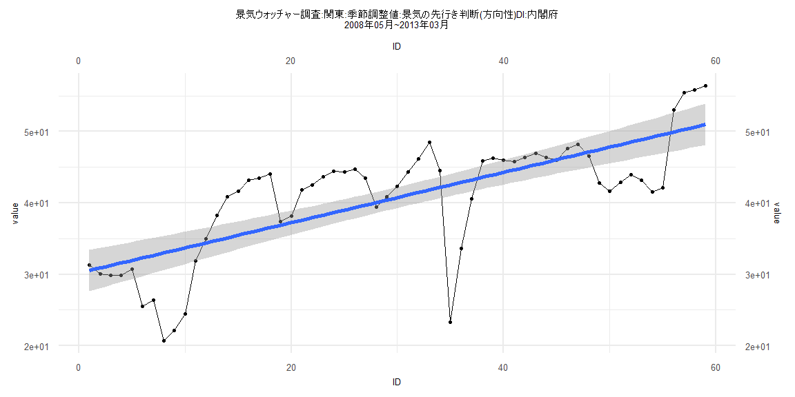
Call:
lm(formula = value ~ ID)

Residuals:
    Min      1Q  Median      3Q     Max
-19.218  -2.388   1.166   4.394   7.579

Coefficients:
            Estimate Std. Error t value             Pr(>|t|)
(Intercept) 30.17236    1.48305  20.345 < 0.0000000000000002 ***
ID           0.35273    0.04299   8.205      0.0000000000315 ***
---
Signif. codes:  0 '***' 0.001 '**' 0.01 '*' 0.05 '.' 0.1 ' ' 1

Residual standard error: 5.624 on 57 degrees of freedom
Multiple R-squared:  0.5415,    Adjusted R-squared:  0.5334
F-statistic: 67.32 on 1 and 57 DF,  p-value: 0.00000000003145


    Two-sample Kolmogorov-Smirnov test

data:  lm_residuals and rnorm(n = length(lm_residuals), mean = 0, sd = sd(lm_residuals))
D = 0.15254, p-value = 0.5021
alternative hypothesis: two-sided


    Durbin-Watson test

data:  value ~ ID
DW = 0.57963, p-value = 0.00000000001725
alternative hypothesis: true autocorrelation is greater than 0


    studentized Breusch-Pagan test

data:  value ~ ID
BP = 0.21436, df = 1, p-value = 0.6434


    Box-Ljung test

data:  lm_residuals
X-squared = 30.569, df = 1, p-value = 0.00000003222
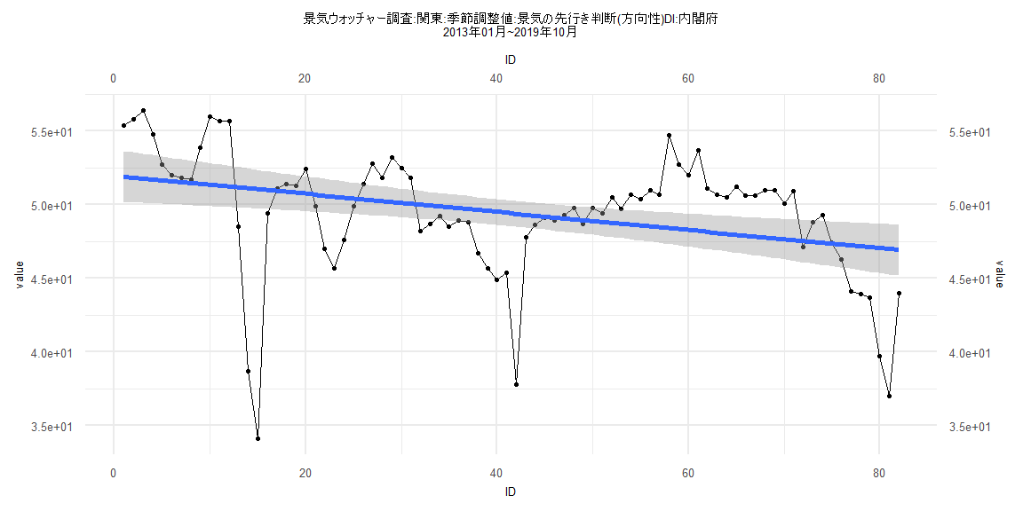
Call:
lm(formula = value ~ ID)

Residuals:
     Min       1Q   Median       3Q      Max
-16.4588  -1.1666   0.8829   2.5050   6.2804

Coefficients:
            Estimate Std. Error t value            Pr(>|t|)
(Intercept) 51.15579    0.90319  56.639 <0.0000000000000002 ***
ID          -0.04975    0.01962  -2.536              0.0132 *
---
Signif. codes:  0 '***' 0.001 '**' 0.01 '*' 0.05 '.' 0.1 ' ' 1

Residual standard error: 3.976 on 77 degrees of freedom
Multiple R-squared:  0.07709,   Adjusted R-squared:  0.06511
F-statistic: 6.432 on 1 and 77 DF,  p-value: 0.01323


    Two-sample Kolmogorov-Smirnov test

data:  lm_residuals and rnorm(n = length(lm_residuals), mean = 0, sd = sd(lm_residuals))
D = 0.22785, p-value = 0.03278
alternative hypothesis: two-sided


    Durbin-Watson test

data:  value ~ ID
DW = 0.6343, p-value = 0.0000000000003033
alternative hypothesis: true autocorrelation is greater than 0


    studentized Breusch-Pagan test

data:  value ~ ID
BP = 0.46572, df = 1, p-value = 0.495


    Box-Ljung test

data:  lm_residuals
X-squared = 37.154, df = 1, p-value = 0.000000001091