Analysis
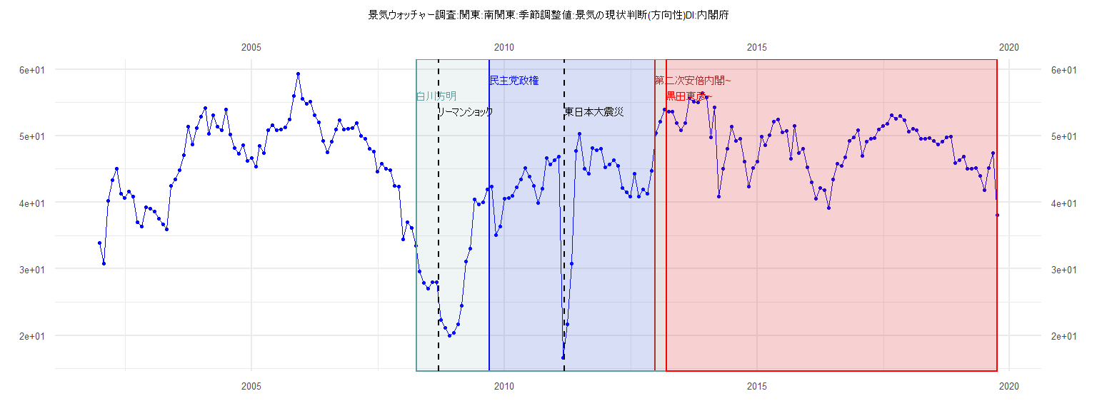
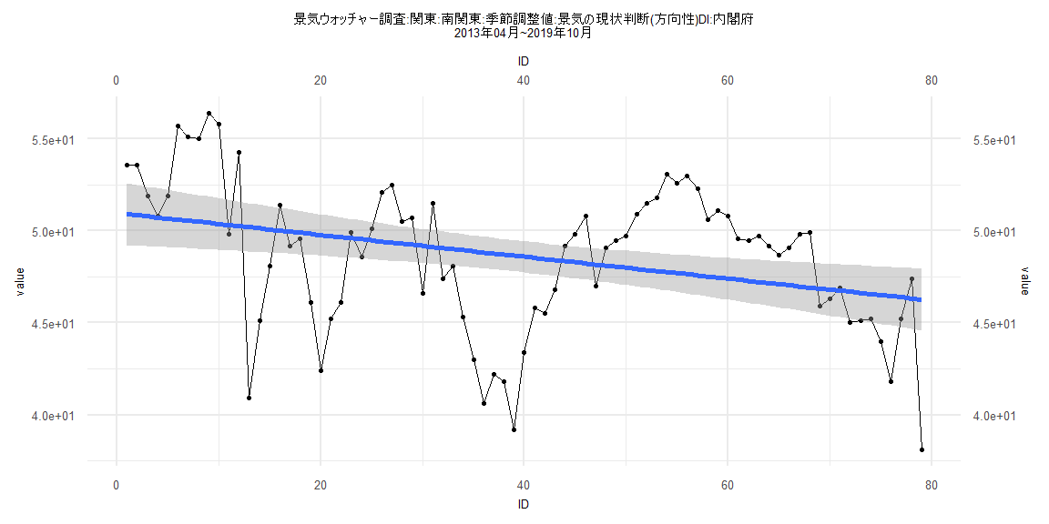
[1] "景気ウォッチャー調査:関東:南関東:季節調整値:景気の現状判断(方向性)DI:内閣府"
      Jan  Feb  Mar  Apr  May  Jun  Jul  Aug  Sep  Oct  Nov  Dec
2002 33.9 30.8 40.2 43.3 45.0 41.3 40.7 41.6 40.9 37.0 36.4 39.3
2003 39.0 38.6 37.5 36.7 35.9 42.5 43.4 44.8 47.1 51.4 48.7 51.2
2004 52.9 54.2 50.3 53.1 51.4 50.8 54.0 50.2 48.2 47.3 48.6 46.2
2005 46.7 45.4 48.5 47.4 50.8 51.6 50.8 50.9 51.3 52.4 56.0 59.3
2006 55.6 54.8 55.1 53.1 52.0 49.2 47.5 49.1 51.0 52.3 51.0 51.1
2007 51.2 51.9 50.0 49.5 48.0 47.6 44.6 45.8 45.1 44.8 42.5 42.4
2008 34.4 37.0 36.2 33.5 29.6 27.9 27.0 28.0 28.0 22.3 21.1 20.0
2009 20.4 21.7 24.5 31.1 33.0 40.4 39.7 40.0 41.9 42.4 35.1 36.4
2010 40.6 40.7 41.0 42.3 43.4 45.2 43.9 42.5 39.9 42.1 46.7 45.7
2011 46.3 46.9 16.7 21.7 30.8 47.7 50.3 45.0 44.3 48.2 47.8 48.0
2012 45.3 45.7 46.3 45.5 42.2 41.5 40.9 44.3 40.9 41.9 41.3 44.7
2013 50.4 52.1 54.0 53.6 53.6 51.9 50.8 51.9 55.7 55.1 55.0 56.4
2014 55.8 49.8 54.3 40.9 45.1 48.1 51.4 49.2 49.6 46.1 42.4 45.2
2015 46.1 49.9 48.6 50.1 52.1 52.5 50.5 50.7 46.6 51.5 47.4 48.1
2016 45.3 43.0 40.6 42.2 41.8 39.2 43.4 45.8 45.5 46.8 49.2 49.8
2017 50.8 47.0 49.1 49.5 49.7 50.9 51.5 51.8 53.1 52.6 53.0 52.3
2018 50.6 51.1 50.8 49.6 49.5 49.7 49.2 48.7 49.1 49.8 49.9 45.9
2019 46.3 46.9 45.0 45.1 45.2 44.0 41.8 45.2 47.4 38.1
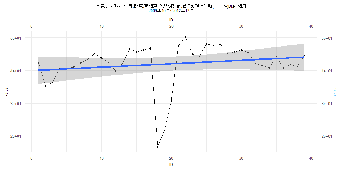
Call:
lm(formula = value ~ ID)

Residuals:
    Min      1Q  Median      3Q     Max
-25.194  -1.669   1.565   3.631   7.984

Coefficients:
            Estimate Std. Error t value            Pr(>|t|)
(Intercept) 39.99744    2.14703  18.629 <0.0000000000000002 ***
ID           0.10538    0.09356   1.126               0.267
---
Signif. codes:  0 '***' 0.001 '**' 0.01 '*' 0.05 '.' 0.1 ' ' 1

Residual standard error: 6.576 on 37 degrees of freedom
Multiple R-squared:  0.03316,   Adjusted R-squared:  0.007026
F-statistic: 1.269 on 1 and 37 DF,  p-value: 0.2672


    Two-sample Kolmogorov-Smirnov test

data:  lm_residuals and rnorm(n = length(lm_residuals), mean = 0, sd = sd(lm_residuals))
D = 0.25641, p-value = 0.1547
alternative hypothesis: two-sided


    Durbin-Watson test

data:  value ~ ID
DW = 0.95596, p-value = 0.00009253
alternative hypothesis: true autocorrelation is greater than 0


    studentized Breusch-Pagan test

data:  value ~ ID
BP = 0.052948, df = 1, p-value = 0.818


    Box-Ljung test

data:  lm_residuals
X-squared = 11.389, df = 1, p-value = 0.0007386
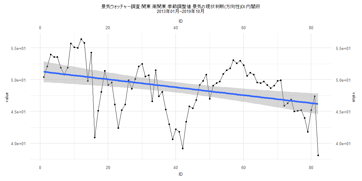
Call:
lm(formula = value ~ ID)

Residuals:
    Min      1Q  Median      3Q     Max
-9.4920 -1.7070  0.9382  2.5998  5.8371

Coefficients:
            Estimate Std. Error t value             Pr(>|t|)
(Intercept) 51.31120    0.83312  61.589 < 0.0000000000000002 ***
ID          -0.06236    0.01744  -3.576             0.000595 ***
---
Signif. codes:  0 '***' 0.001 '**' 0.01 '*' 0.05 '.' 0.1 ' ' 1

Residual standard error: 3.738 on 80 degrees of freedom
Multiple R-squared:  0.1378,    Adjusted R-squared:  0.1271
F-statistic: 12.79 on 1 and 80 DF,  p-value: 0.0005951


    Two-sample Kolmogorov-Smirnov test

data:  lm_residuals and rnorm(n = length(lm_residuals), mean = 0, sd = sd(lm_residuals))
D = 0.12195, p-value = 0.5785
alternative hypothesis: two-sided


    Durbin-Watson test

data:  value ~ ID
DW = 0.57705, p-value = 0.000000000000004157
alternative hypothesis: true autocorrelation is greater than 0


    studentized Breusch-Pagan test

data:  value ~ ID
BP = 0.37021, df = 1, p-value = 0.5429


    Box-Ljung test

data:  lm_residuals
X-squared = 39.532, df = 1, p-value = 0.0000000003228
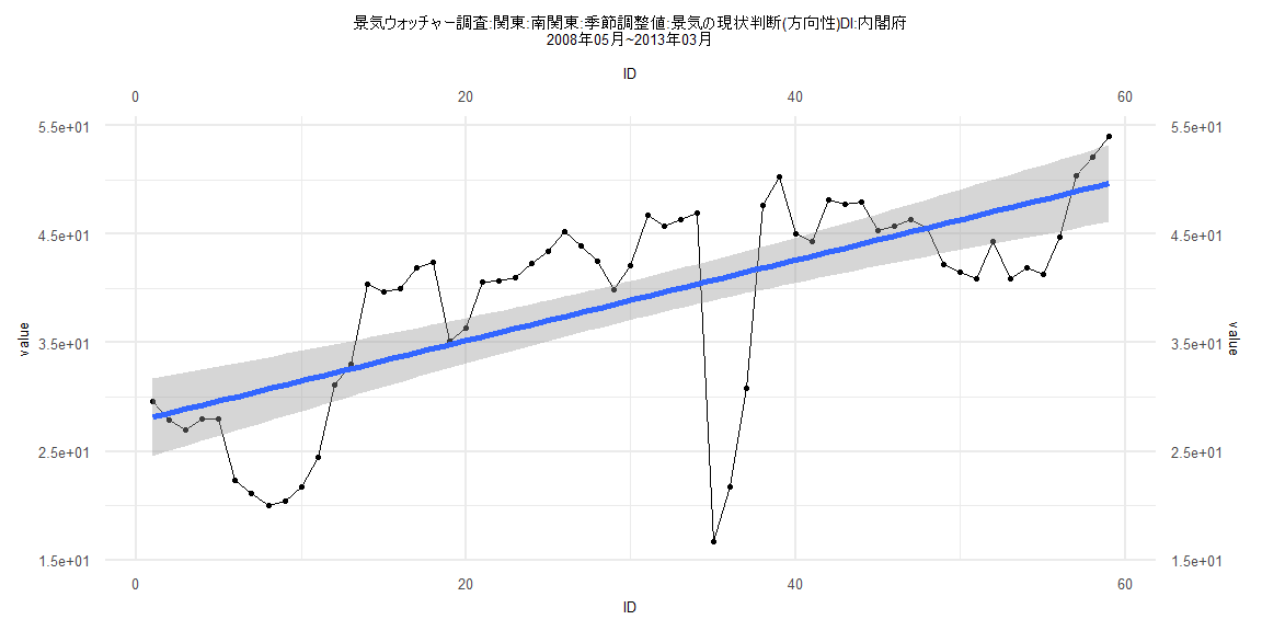
Call:
lm(formula = value ~ ID)

Residuals:
    Min      1Q  Median      3Q     Max
-24.057  -3.800   1.317   5.331   8.059

Coefficients:
            Estimate Std. Error t value             Pr(>|t|)
(Intercept) 27.77049    1.82339   15.23 < 0.0000000000000002 ***
ID           0.37104    0.05286    7.02        0.00000000295 ***
---
Signif. codes:  0 '***' 0.001 '**' 0.01 '*' 0.05 '.' 0.1 ' ' 1

Residual standard error: 6.914 on 57 degrees of freedom
Multiple R-squared:  0.4637,    Adjusted R-squared:  0.4542
F-statistic: 49.28 on 1 and 57 DF,  p-value: 0.000000002951


    Two-sample Kolmogorov-Smirnov test

data:  lm_residuals and rnorm(n = length(lm_residuals), mean = 0, sd = sd(lm_residuals))
D = 0.22034, p-value = 0.1141
alternative hypothesis: two-sided


    Durbin-Watson test

data:  value ~ ID
DW = 0.62911, p-value = 0.0000000001436
alternative hypothesis: true autocorrelation is greater than 0


    studentized Breusch-Pagan test

data:  value ~ ID
BP = 0.053371, df = 1, p-value = 0.8173


    Box-Ljung test

data:  lm_residuals
X-squared = 28.828, df = 1, p-value = 0.0000000791
Call:
lm(formula = value ~ ID)

Residuals:
    Min      1Q  Median      3Q     Max
-9.4519 -1.8341  0.9837  2.7162  5.9625

Coefficients:
            Estimate Std. Error t value             Pr(>|t|)
(Intercept) 50.97313    0.86148  59.169 < 0.0000000000000002 ***
ID          -0.05952    0.01871  -3.181              0.00212 **
---
Signif. codes:  0 '***' 0.001 '**' 0.01 '*' 0.05 '.' 0.1 ' ' 1

Residual standard error: 3.792 on 77 degrees of freedom
Multiple R-squared:  0.1162,    Adjusted R-squared:  0.1047
F-statistic: 10.12 on 1 and 77 DF,  p-value: 0.002116


    Two-sample Kolmogorov-Smirnov test

data:  lm_residuals and rnorm(n = length(lm_residuals), mean = 0, sd = sd(lm_residuals))
D = 0.12658, p-value = 0.5543
alternative hypothesis: two-sided


    Durbin-Watson test

data:  value ~ ID
DW = 0.57607, p-value = 0.00000000000001144
alternative hypothesis: true autocorrelation is greater than 0


    studentized Breusch-Pagan test

data:  value ~ ID
BP = 0.99138, df = 1, p-value = 0.3194


    Box-Ljung test

data:  lm_residuals
X-squared = 37.774, df = 1, p-value = 0.0000000007944