Analysis
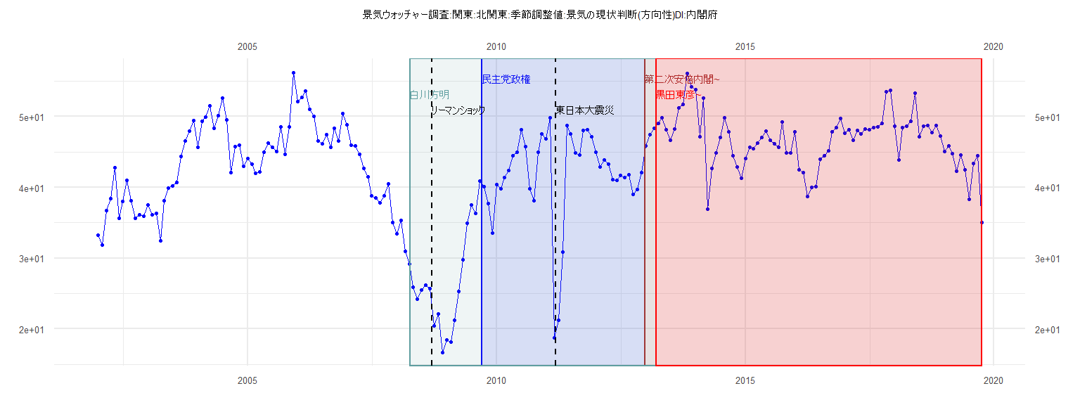
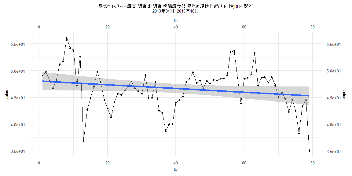
[1] "景気ウォッチャー調査:関東:北関東:季節調整値:景気の現状判断(方向性)DI:内閣府"
      Jan  Feb  Mar  Apr  May  Jun  Jul  Aug  Sep  Oct  Nov  Dec
2002 33.3 31.9 36.7 38.4 42.8 35.6 38.0 41.0 38.1 35.6 36.1 35.9
2003 37.5 36.1 36.3 32.5 38.1 39.9 40.2 40.7 44.4 46.6 48.0 49.4
2004 45.7 49.3 49.9 51.5 48.4 50.1 52.6 49.5 42.1 45.8 46.0 43.0
2005 44.1 43.3 42.0 42.2 45.0 46.3 45.7 45.1 48.6 44.7 48.6 56.2
2006 52.1 52.7 53.6 51.0 50.0 46.6 46.2 47.5 45.7 48.4 46.6 50.4
2007 48.9 46.0 45.9 44.7 42.7 41.5 38.8 38.5 37.8 38.8 40.5 35.0
2008 33.4 35.3 31.0 29.2 25.9 24.2 25.5 26.2 25.7 20.4 22.1 16.7
2009 18.4 18.1 21.2 25.3 29.8 34.9 37.5 36.3 40.9 40.1 37.7 33.5
2010 40.4 39.8 41.4 42.4 44.5 45.0 48.2 45.8 39.8 38.1 45.0 47.6
2011 46.9 49.8 18.7 21.2 30.9 48.8 47.6 44.9 44.6 48.1 48.2 47.2
2012 45.0 42.9 43.9 43.3 41.1 41.0 41.7 41.4 41.8 39.0 39.7 42.1
2013 45.9 47.5 48.4 49.1 49.8 48.2 46.7 48.3 51.2 51.7 56.1 54.2
2014 53.8 47.2 52.6 36.9 42.7 44.9 47.1 49.8 47.9 44.5 42.9 41.3
2015 44.1 45.7 45.5 46.3 47.1 48.0 46.7 46.2 45.7 49.2 44.9 44.9
2016 47.9 42.5 42.1 38.7 40.0 40.1 44.0 44.5 45.2 47.9 48.5 49.7
2017 47.7 48.2 46.7 48.1 47.6 48.3 48.2 48.5 48.6 49.1 53.5 53.7
2018 48.7 43.9 48.5 48.7 49.3 53.3 47.2 48.7 48.8 47.8 48.8 47.3
2019 45.1 45.9 44.8 42.3 44.6 42.5 38.3 43.4 44.5 35.0
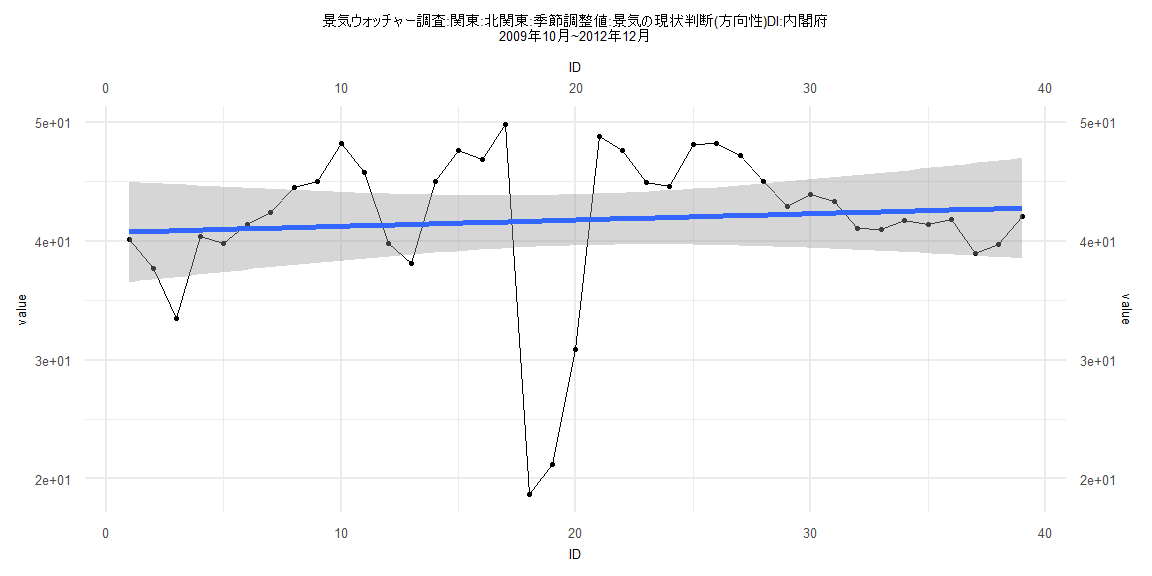
Call:
lm(formula = value ~ ID)

Residuals:
     Min       1Q   Median       3Q      Max
-22.9666  -1.3792   0.6549   4.1541   8.1860

Coefficients:
            Estimate Std. Error t value            Pr(>|t|)
(Intercept) 40.71997    2.16445  18.813 <0.0000000000000002 ***
ID           0.05259    0.09431   0.558                0.58
---
Signif. codes:  0 '***' 0.001 '**' 0.01 '*' 0.05 '.' 0.1 ' ' 1

Residual standard error: 6.629 on 37 degrees of freedom
Multiple R-squared:  0.008334,  Adjusted R-squared:  -0.01847
F-statistic: 0.3109 on 1 and 37 DF,  p-value: 0.5805


    Two-sample Kolmogorov-Smirnov test

data:  lm_residuals and rnorm(n = length(lm_residuals), mean = 0, sd = sd(lm_residuals))
D = 0.25641, p-value = 0.1547
alternative hypothesis: two-sided


    Durbin-Watson test

data:  value ~ ID
DW = 1.0074, p-value = 0.000205
alternative hypothesis: true autocorrelation is greater than 0


    studentized Breusch-Pagan test

data:  value ~ ID
BP = 0.15958, df = 1, p-value = 0.6895


    Box-Ljung test

data:  lm_residuals
X-squared = 10.352, df = 1, p-value = 0.001293
Call:
lm(formula = value ~ ID)

Residuals:
     Min       1Q   Median       3Q      Max
-10.6368  -2.0383   0.3216   2.2654   8.3998

Coefficients:
            Estimate Std. Error t value            Pr(>|t|)
(Intercept) 48.05962    0.84350  56.977 <0.0000000000000002 ***
ID          -0.03267    0.01766  -1.851              0.0679 .
---
Signif. codes:  0 '***' 0.001 '**' 0.01 '*' 0.05 '.' 0.1 ' ' 1

Residual standard error: 3.784 on 80 degrees of freedom
Multiple R-squared:  0.04105,   Adjusted R-squared:  0.02907
F-statistic: 3.425 on 1 and 80 DF,  p-value: 0.06791


    Two-sample Kolmogorov-Smirnov test

data:  lm_residuals and rnorm(n = length(lm_residuals), mean = 0, sd = sd(lm_residuals))
D = 0.14634, p-value = 0.3453
alternative hypothesis: two-sided


    Durbin-Watson test

data:  value ~ ID
DW = 0.76038, p-value = 0.00000000005549
alternative hypothesis: true autocorrelation is greater than 0


    studentized Breusch-Pagan test

data:  value ~ ID
BP = 0.047283, df = 1, p-value = 0.8279


    Box-Ljung test

data:  lm_residuals
X-squared = 27.707, df = 1, p-value = 0.0000001411
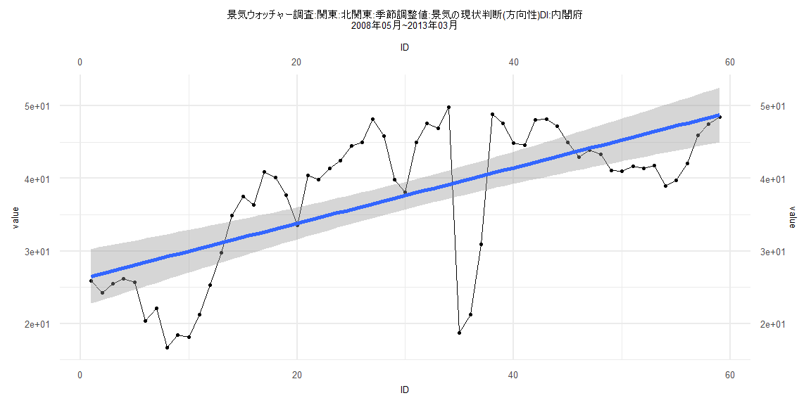
Call:
lm(formula = value ~ ID)

Residuals:
     Min       1Q   Median       3Q      Max
-20.8430  -4.4655  -0.2953   6.0481  11.7224

Coefficients:
            Estimate Std. Error t value             Pr(>|t|)
(Intercept) 26.13174    1.92811  13.553 < 0.0000000000000002 ***
ID           0.38318    0.05589   6.856        0.00000000554 ***
---
Signif. codes:  0 '***' 0.001 '**' 0.01 '*' 0.05 '.' 0.1 ' ' 1

Residual standard error: 7.311 on 57 degrees of freedom
Multiple R-squared:  0.4519,    Adjusted R-squared:  0.4423
F-statistic:    47 on 1 and 57 DF,  p-value: 0.000000005535


    Two-sample Kolmogorov-Smirnov test

data:  lm_residuals and rnorm(n = length(lm_residuals), mean = 0, sd = sd(lm_residuals))
D = 0.10169, p-value = 0.9239
alternative hypothesis: two-sided


    Durbin-Watson test

data:  value ~ ID
DW = 0.59679, p-value = 0.00000000003685
alternative hypothesis: true autocorrelation is greater than 0


    studentized Breusch-Pagan test

data:  value ~ ID
BP = 0.29517, df = 1, p-value = 0.5869


    Box-Ljung test

data:  lm_residuals
X-squared = 30.538, df = 1, p-value = 0.00000003274
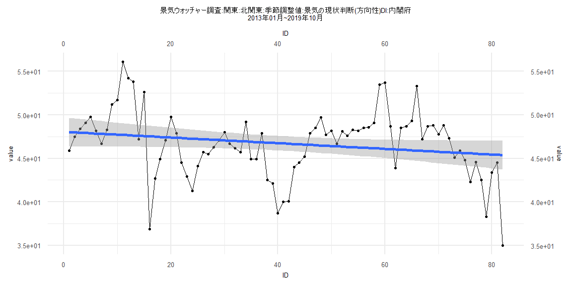
Call:
lm(formula = value ~ ID)

Residuals:
     Min       1Q   Median       3Q      Max
-10.7250  -2.0441   0.3001   2.2931   8.3004

Coefficients:
            Estimate Std. Error t value            Pr(>|t|)
(Intercept) 48.07887    0.87425  54.994 <0.0000000000000002 ***
ID          -0.03491    0.01899  -1.839              0.0698 .
---
Signif. codes:  0 '***' 0.001 '**' 0.01 '*' 0.05 '.' 0.1 ' ' 1

Residual standard error: 3.848 on 77 degrees of freedom
Multiple R-squared:  0.04207,   Adjusted R-squared:  0.02963
F-statistic: 3.381 on 1 and 77 DF,  p-value: 0.0698


    Two-sample Kolmogorov-Smirnov test

data:  lm_residuals and rnorm(n = length(lm_residuals), mean = 0, sd = sd(lm_residuals))
D = 0.17722, p-value = 0.1677
alternative hypothesis: two-sided


    Durbin-Watson test

data:  value ~ ID
DW = 0.76024, p-value = 0.0000000001158
alternative hypothesis: true autocorrelation is greater than 0


    studentized Breusch-Pagan test

data:  value ~ ID
BP = 0.0088582, df = 1, p-value = 0.925


    Box-Ljung test

data:  lm_residuals
X-squared = 26.906, df = 1, p-value = 0.0000002136