Analysis
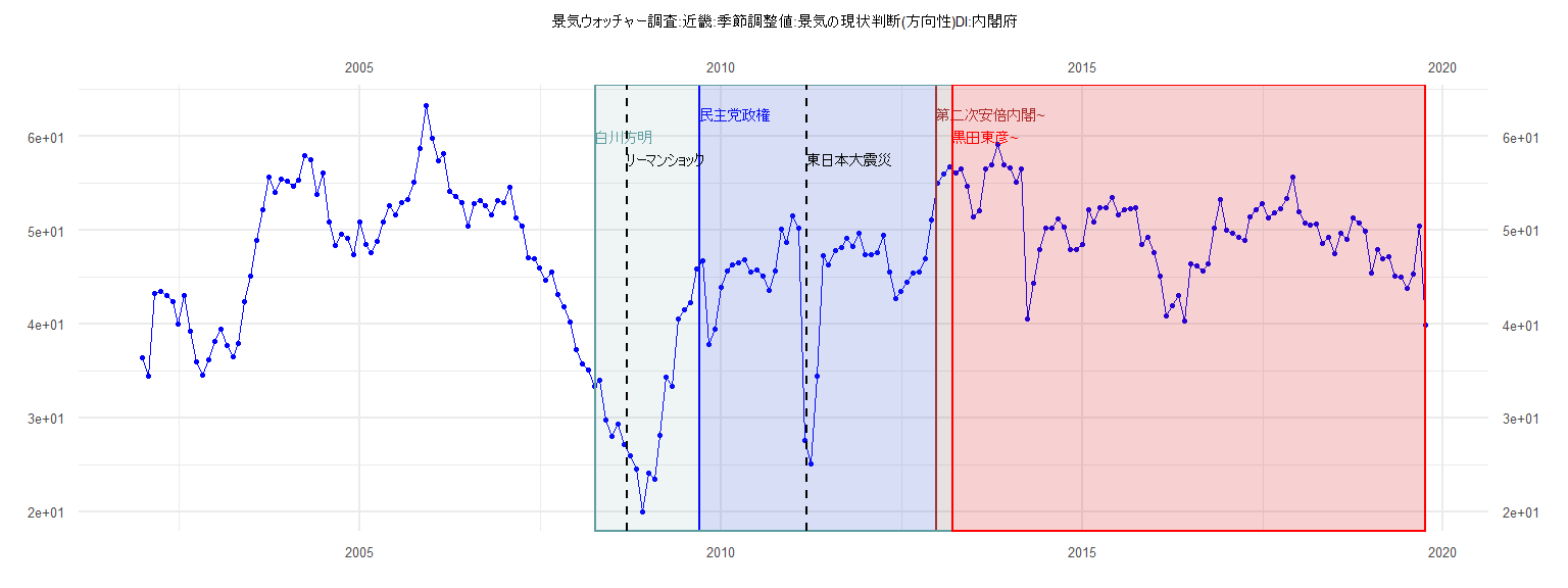
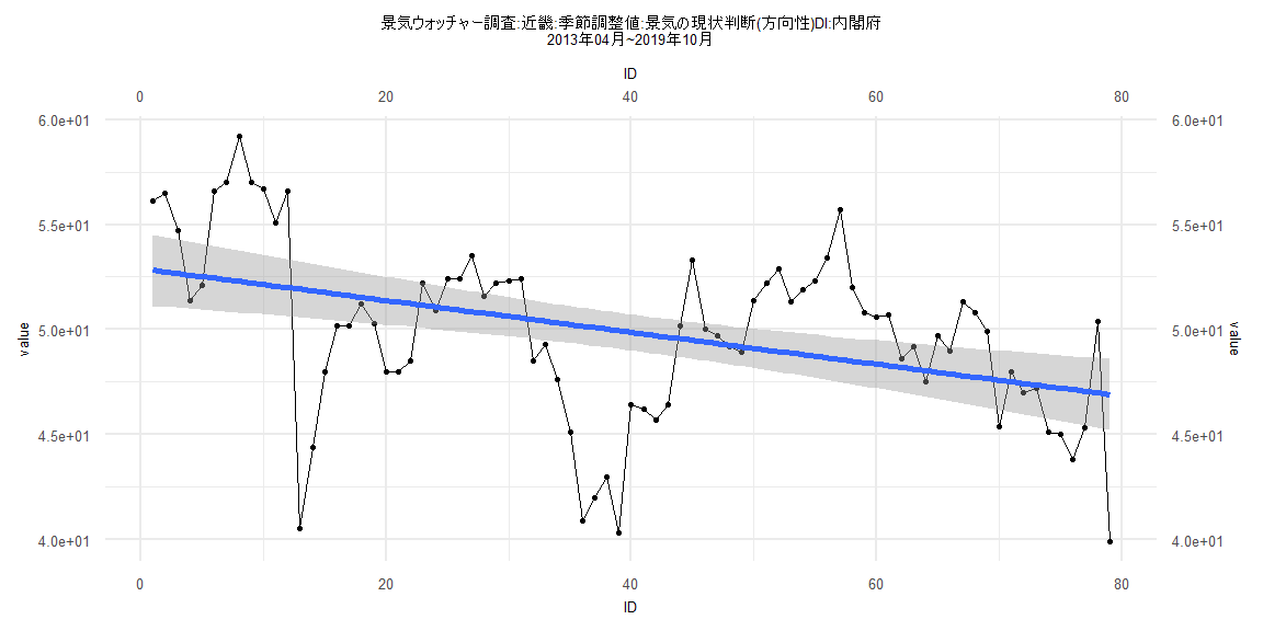
[1] "景気ウォッチャー調査:近畿:季節調整値:景気の現状判断(方向性)DI:内閣府"
      Jan  Feb  Mar  Apr  May  Jun  Jul  Aug  Sep  Oct  Nov  Dec
2002 36.4 34.4 43.3 43.5 43.0 42.4 40.0 43.0 39.2 36.0 34.5 36.2
2003 38.1 39.5 37.7 36.5 37.9 42.4 45.1 48.9 52.2 55.7 54.1 55.5
2004 55.2 54.7 55.4 58.0 57.5 53.8 56.1 50.9 48.4 49.6 49.1 47.4
2005 50.9 48.5 47.6 48.8 50.9 52.6 51.6 53.0 53.3 55.1 58.7 63.3
2006 59.8 57.4 58.2 54.2 53.6 53.0 50.5 52.9 53.2 52.6 51.7 53.2
2007 53.0 54.6 51.3 50.5 47.1 47.0 46.0 44.7 45.6 43.2 41.9 40.2
2008 37.3 35.7 35.1 33.4 34.0 29.8 28.0 29.3 27.1 25.9 24.5 20.0
2009 24.1 23.4 28.1 34.3 33.3 40.5 41.5 42.3 45.9 46.7 37.8 39.5
2010 43.9 45.7 46.3 46.5 46.9 45.5 45.8 45.1 43.6 45.7 50.1 48.7
2011 51.5 50.2 27.6 25.1 34.4 47.3 46.3 47.8 48.2 49.1 48.3 49.7
2012 47.4 47.4 47.6 49.5 45.6 42.7 43.5 44.5 45.4 45.6 47.0 51.1
2013 55.0 56.0 56.8 56.1 56.5 54.7 51.4 52.1 56.6 57.0 59.2 57.0
2014 56.7 55.1 56.6 40.5 44.4 48.0 50.2 50.2 51.2 50.3 48.0 48.0
2015 48.5 52.2 50.9 52.4 52.4 53.5 51.6 52.2 52.3 52.4 48.5 49.3
2016 47.6 45.1 40.9 42.0 43.0 40.3 46.4 46.2 45.7 46.4 50.2 53.3
2017 50.0 49.7 49.2 48.9 51.4 52.2 52.9 51.3 51.9 52.3 53.4 55.7
2018 52.0 50.8 50.6 50.7 48.6 49.2 47.5 49.7 49.0 51.3 50.8 49.9
2019 45.4 48.0 47.0 47.2 45.1 45.0 43.8 45.3 50.4 39.9
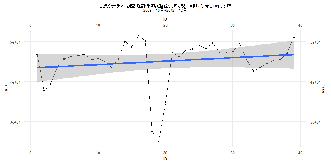
Call:
lm(formula = value ~ ID)

Residuals:
     Min       1Q   Median       3Q      Max
-19.9573  -0.9318   1.5192   2.7515   6.7015

Coefficients:
            Estimate Std. Error t value            Pr(>|t|)
(Intercept) 43.41808    1.81510  23.921 <0.0000000000000002 ***
ID           0.08628    0.07909   1.091               0.282
---
Signif. codes:  0 '***' 0.001 '**' 0.01 '*' 0.05 '.' 0.1 ' ' 1

Residual standard error: 5.559 on 37 degrees of freedom
Multiple R-squared:  0.03116,   Adjusted R-squared:  0.004972
F-statistic:  1.19 on 1 and 37 DF,  p-value: 0.2824


    Two-sample Kolmogorov-Smirnov test

data:  lm_residuals and rnorm(n = length(lm_residuals), mean = 0, sd = sd(lm_residuals))
D = 0.25641, p-value = 0.1547
alternative hypothesis: two-sided


    Durbin-Watson test

data:  value ~ ID
DW = 0.85307, p-value = 0.00001542
alternative hypothesis: true autocorrelation is greater than 0


    studentized Breusch-Pagan test

data:  value ~ ID
BP = 0.10741, df = 1, p-value = 0.7431


    Box-Ljung test

data:  lm_residuals
X-squared = 13.236, df = 1, p-value = 0.0002746
Call:
lm(formula = value ~ ID)

Residuals:
     Min       1Q   Median       3Q      Max
-11.7161  -2.0314   0.6338   2.6911   7.1605

Coefficients:
            Estimate Std. Error t value             Pr(>|t|)
(Intercept) 53.55303    0.84704  63.224 < 0.0000000000000002 ***
ID          -0.08356    0.01773  -4.713            0.0000102 ***
---
Signif. codes:  0 '***' 0.001 '**' 0.01 '*' 0.05 '.' 0.1 ' ' 1

Residual standard error: 3.8 on 80 degrees of freedom
Multiple R-squared:  0.2173,    Adjusted R-squared:  0.2075
F-statistic: 22.21 on 1 and 80 DF,  p-value: 0.00001016


    Two-sample Kolmogorov-Smirnov test

data:  lm_residuals and rnorm(n = length(lm_residuals), mean = 0, sd = sd(lm_residuals))
D = 0.15854, p-value = 0.2552
alternative hypothesis: two-sided


    Durbin-Watson test

data:  value ~ ID
DW = 0.62473, p-value = 0.00000000000006865
alternative hypothesis: true autocorrelation is greater than 0


    studentized Breusch-Pagan test

data:  value ~ ID
BP = 1.1647, df = 1, p-value = 0.2805


    Box-Ljung test

data:  lm_residuals
X-squared = 37.787, df = 1, p-value = 0.0000000007892
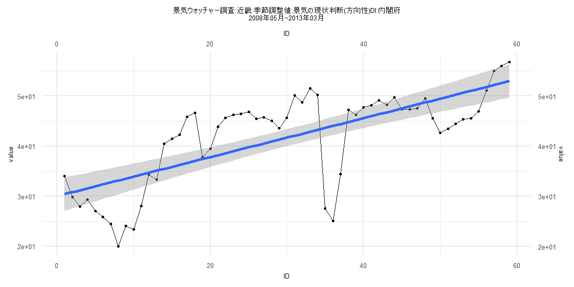
Call:
lm(formula = value ~ ID)

Residuals:
    Min      1Q  Median      3Q     Max
-18.937  -4.652   1.539   5.146   9.668

Coefficients:
            Estimate Std. Error t value             Pr(>|t|)
(Intercept) 30.02624    1.71368  17.521 < 0.0000000000000002 ***
ID           0.38918    0.04968   7.834        0.00000000013 ***
---
Signif. codes:  0 '***' 0.001 '**' 0.01 '*' 0.05 '.' 0.1 ' ' 1

Residual standard error: 6.498 on 57 degrees of freedom
Multiple R-squared:  0.5185,    Adjusted R-squared:   0.51
F-statistic: 61.38 on 1 and 57 DF,  p-value: 0.0000000001296


    Two-sample Kolmogorov-Smirnov test

data:  lm_residuals and rnorm(n = length(lm_residuals), mean = 0, sd = sd(lm_residuals))
D = 0.10169, p-value = 0.9239
alternative hypothesis: two-sided


    Durbin-Watson test

data:  value ~ ID
DW = 0.49058, p-value = 0.0000000000002056
alternative hypothesis: true autocorrelation is greater than 0


    studentized Breusch-Pagan test

data:  value ~ ID
BP = 0.88974, df = 1, p-value = 0.3455


    Box-Ljung test

data:  lm_residuals
X-squared = 34.813, df = 1, p-value = 0.000000003629
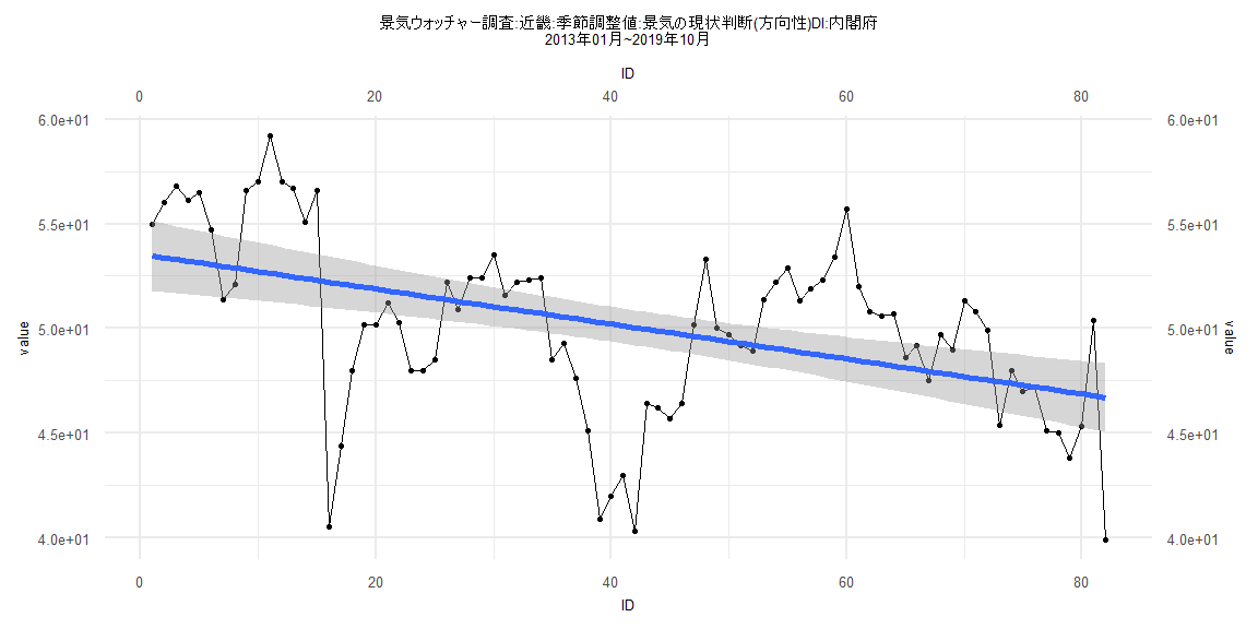
Call:
lm(formula = value ~ ID)

Residuals:
     Min       1Q   Median       3Q      Max
-11.4147  -2.1820   0.5926   2.8412   7.1283

Coefficients:
            Estimate Std. Error t value             Pr(>|t|)
(Intercept) 52.90243    0.87055  60.769 < 0.0000000000000002 ***
ID          -0.07598    0.01891  -4.019             0.000135 ***
---
Signif. codes:  0 '***' 0.001 '**' 0.01 '*' 0.05 '.' 0.1 ' ' 1

Residual standard error: 3.832 on 77 degrees of freedom
Multiple R-squared:  0.1734,    Adjusted R-squared:  0.1626
F-statistic: 16.15 on 1 and 77 DF,  p-value: 0.0001353


    Two-sample Kolmogorov-Smirnov test

data:  lm_residuals and rnorm(n = length(lm_residuals), mean = 0, sd = sd(lm_residuals))
D = 0.12658, p-value = 0.5543
alternative hypothesis: two-sided


    Durbin-Watson test

data:  value ~ ID
DW = 0.63634, p-value = 0.0000000000003379
alternative hypothesis: true autocorrelation is greater than 0


    studentized Breusch-Pagan test

data:  value ~ ID
BP = 1.9765, df = 1, p-value = 0.1598


    Box-Ljung test

data:  lm_residuals
X-squared = 35.242, df = 1, p-value = 0.000000002912