Analysis
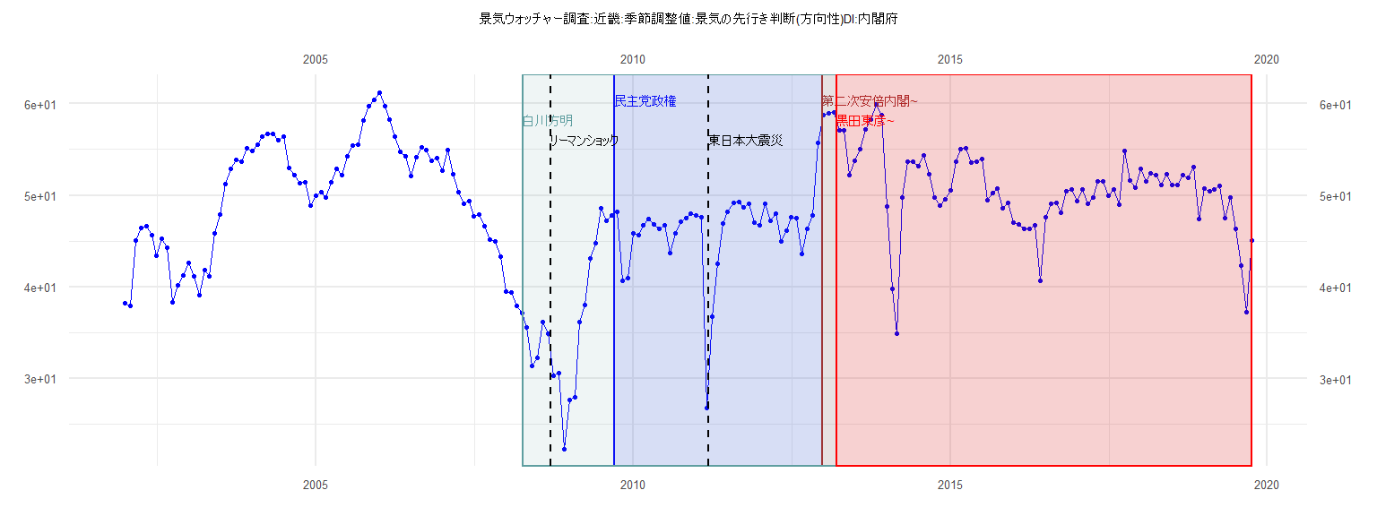
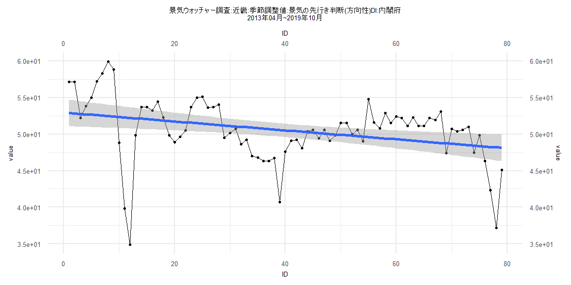
[1] "景気ウォッチャー調査:近畿:季節調整値:景気の先行き判断(方向性)DI:内閣府"
      Jan  Feb  Mar  Apr  May  Jun  Jul  Aug  Sep  Oct  Nov  Dec
2002 38.2 37.9 45.1 46.4 46.6 45.6 43.4 45.3 44.3 38.3 40.2 41.2
2003 42.6 41.1 39.1 41.8 41.1 45.8 47.9 51.2 52.9 53.9 53.7 55.1
2004 54.8 55.5 56.4 56.7 56.7 56.0 56.4 53.0 52.2 51.3 51.4 48.9
2005 50.0 50.3 49.8 51.4 52.9 52.2 54.3 55.4 55.5 58.2 59.7 60.4
2006 61.2 59.7 58.3 56.4 54.7 54.3 52.1 54.2 55.2 54.9 53.8 54.1
2007 52.7 54.9 52.3 50.3 49.1 49.4 47.7 47.9 46.6 45.2 45.0 43.3
2008 39.5 39.4 37.9 37.1 35.6 31.4 32.2 36.2 34.9 30.3 30.6 22.3
2009 27.6 27.9 36.2 38.0 43.1 44.8 48.6 47.2 47.8 48.2 40.7 40.9
2010 45.8 45.6 46.7 47.4 46.8 46.3 46.7 43.7 45.8 47.1 47.5 48.0
2011 47.8 47.6 26.8 36.7 42.5 46.9 48.2 49.2 49.3 48.7 49.1 47.0
2012 46.7 49.1 47.2 48.0 45.0 46.1 47.6 47.5 43.6 46.3 47.8 55.7
2013 58.8 59.0 59.1 57.1 57.1 52.2 53.8 55.0 57.2 58.3 59.9 58.8
2014 48.8 39.8 34.9 49.8 53.7 53.7 53.2 54.4 52.3 49.8 48.9 49.6
2015 50.5 53.7 55.0 55.1 53.6 53.7 54.0 49.5 50.2 50.7 48.6 49.2
2016 47.0 46.8 46.3 46.3 46.7 40.7 47.6 49.1 49.2 48.1 50.4 50.6
2017 49.4 50.6 49.1 49.8 51.5 51.5 50.0 50.6 49.0 54.8 51.6 50.8
2018 52.9 51.5 52.4 52.2 51.1 52.3 51.1 51.1 52.2 51.9 53.1 47.4
2019 50.7 50.4 50.6 51.0 47.5 49.8 46.3 42.3 37.2 45.1
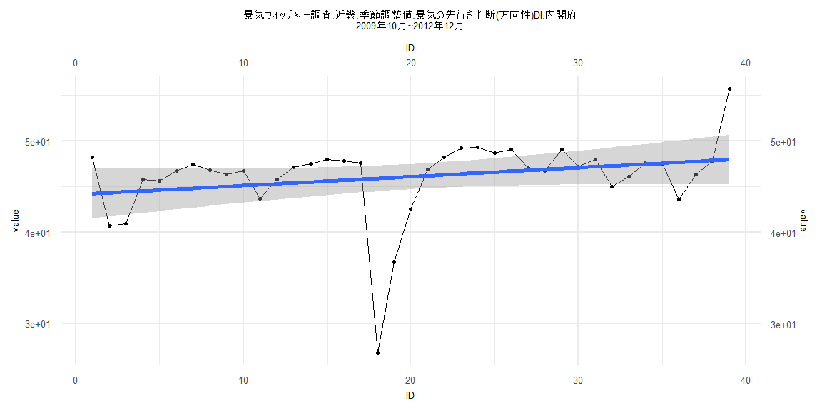
Call:
lm(formula = value ~ ID)

Residuals:
     Min       1Q   Median       3Q      Max
-19.0959  -0.7236   0.9810   2.0488   7.7415

Coefficients:
            Estimate Std. Error t value            Pr(>|t|)
(Intercept) 44.12794    1.38946  31.759 <0.0000000000000002 ***
ID           0.09822    0.06054   1.622               0.113
---
Signif. codes:  0 '***' 0.001 '**' 0.01 '*' 0.05 '.' 0.1 ' ' 1

Residual standard error: 4.255 on 37 degrees of freedom
Multiple R-squared:  0.0664,    Adjusted R-squared:  0.04117
F-statistic: 2.632 on 1 and 37 DF,  p-value: 0.1132


    Two-sample Kolmogorov-Smirnov test

data:  lm_residuals and rnorm(n = length(lm_residuals), mean = 0, sd = sd(lm_residuals))
D = 0.20513, p-value = 0.3888
alternative hypothesis: two-sided


    Durbin-Watson test

data:  value ~ ID
DW = 1.1915, p-value = 0.002251
alternative hypothesis: true autocorrelation is greater than 0


    studentized Breusch-Pagan test

data:  value ~ ID
BP = 0.0040579, df = 1, p-value = 0.9492


    Box-Ljung test

data:  lm_residuals
X-squared = 5.0887, df = 1, p-value = 0.02408
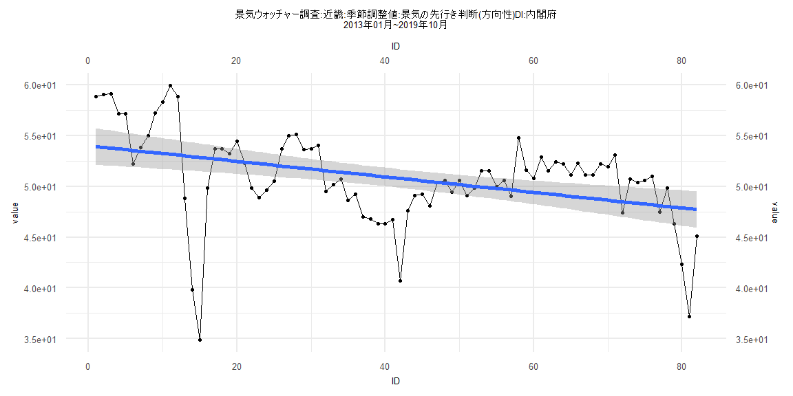
Call:
lm(formula = value ~ ID)

Residuals:
     Min       1Q   Median       3Q      Max
-17.9376  -1.9359   0.7821   2.3760   6.7567

Coefficients:
            Estimate Std. Error t value             Pr(>|t|)
(Intercept) 53.98401    0.92624  58.283 < 0.0000000000000002 ***
ID          -0.07643    0.01939  -3.942             0.000172 ***
---
Signif. codes:  0 '***' 0.001 '**' 0.01 '*' 0.05 '.' 0.1 ' ' 1

Residual standard error: 4.155 on 80 degrees of freedom
Multiple R-squared:  0.1627,    Adjusted R-squared:  0.1522
F-statistic: 15.54 on 1 and 80 DF,  p-value: 0.0001719


    Two-sample Kolmogorov-Smirnov test

data:  lm_residuals and rnorm(n = length(lm_residuals), mean = 0, sd = sd(lm_residuals))
D = 0.14634, p-value = 0.3453
alternative hypothesis: two-sided


    Durbin-Watson test

data:  value ~ ID
DW = 0.64053, p-value = 0.000000000000164
alternative hypothesis: true autocorrelation is greater than 0


    studentized Breusch-Pagan test

data:  value ~ ID
BP = 2.0377, df = 1, p-value = 0.1534


    Box-Ljung test

data:  lm_residuals
X-squared = 38.013, df = 1, p-value = 0.0000000007027
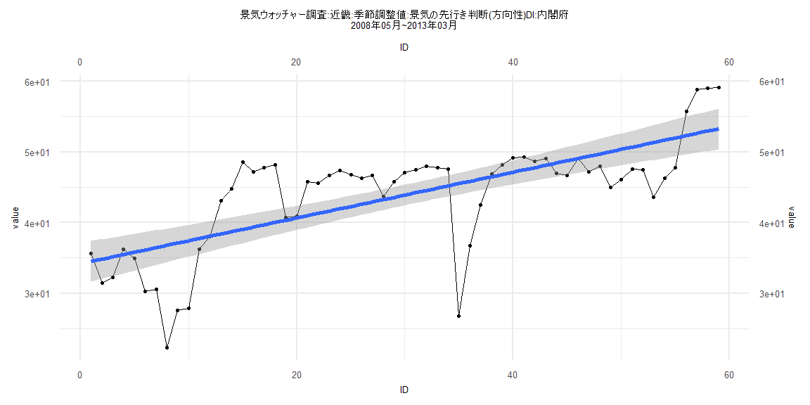
Call:
lm(formula = value ~ ID)

Residuals:
     Min       1Q   Median       3Q      Max
-18.7024  -3.2524   0.7269   3.7476   9.5681

Coefficients:
            Estimate Std. Error t value             Pr(>|t|)
(Intercept) 34.17902    1.47847  23.118 < 0.0000000000000002 ***
ID           0.32352    0.04286   7.549       0.000000000387 ***
---
Signif. codes:  0 '***' 0.001 '**' 0.01 '*' 0.05 '.' 0.1 ' ' 1

Residual standard error: 5.606 on 57 degrees of freedom
Multiple R-squared:  0.4999,    Adjusted R-squared:  0.4911
F-statistic: 56.98 on 1 and 57 DF,  p-value: 0.0000000003874


    Two-sample Kolmogorov-Smirnov test

data:  lm_residuals and rnorm(n = length(lm_residuals), mean = 0, sd = sd(lm_residuals))
D = 0.11864, p-value = 0.8052
alternative hypothesis: two-sided


    Durbin-Watson test

data:  value ~ ID
DW = 0.5985, p-value = 0.00000000003969
alternative hypothesis: true autocorrelation is greater than 0


    studentized Breusch-Pagan test

data:  value ~ ID
BP = 0.82247, df = 1, p-value = 0.3645


    Box-Ljung test

data:  lm_residuals
X-squared = 29.622, df = 1, p-value = 0.00000005252
Call:
lm(formula = value ~ ID)

Residuals:
     Min       1Q   Median       3Q      Max
-17.3123  -1.8574   0.8913   2.3819   7.4434

Coefficients:
            Estimate Std. Error t value             Pr(>|t|)
(Intercept) 52.94508    0.92964  56.952 < 0.0000000000000002 ***
ID          -0.06106    0.02019  -3.024              0.00338 **
---
Signif. codes:  0 '***' 0.001 '**' 0.01 '*' 0.05 '.' 0.1 ' ' 1

Residual standard error: 4.092 on 77 degrees of freedom
Multiple R-squared:  0.1062,    Adjusted R-squared:  0.09457
F-statistic: 9.147 on 1 and 77 DF,  p-value: 0.003384


    Two-sample Kolmogorov-Smirnov test

data:  lm_residuals and rnorm(n = length(lm_residuals), mean = 0, sd = sd(lm_residuals))
D = 0.16456, p-value = 0.2361
alternative hypothesis: two-sided


    Durbin-Watson test

data:  value ~ ID
DW = 0.6834, p-value = 0.000000000003637
alternative hypothesis: true autocorrelation is greater than 0


    studentized Breusch-Pagan test

data:  value ~ ID
BP = 2.0892, df = 1, p-value = 0.1483


    Box-Ljung test

data:  lm_residuals
X-squared = 34.435, df = 1, p-value = 0.000000004408