Analysis
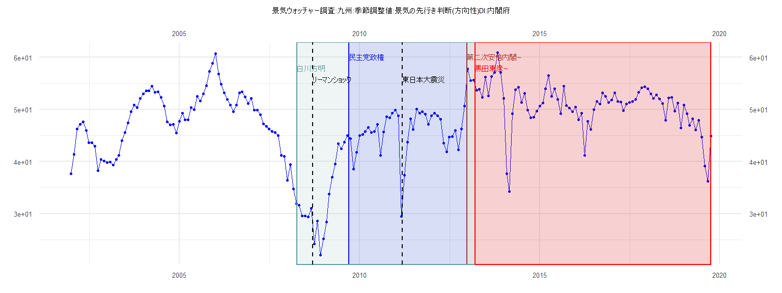
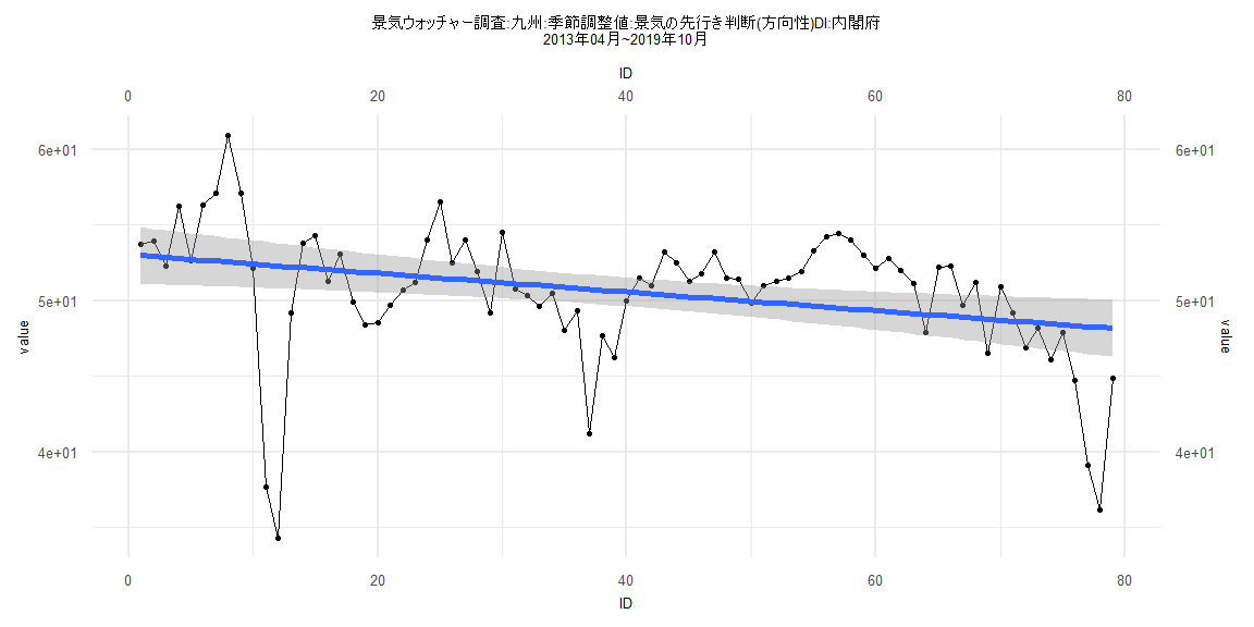
[1] "景気ウォッチャー調査:九州:季節調整値:景気の先行き判断(方向性)DI:内閣府"
      Jan  Feb  Mar  Apr  May  Jun  Jul  Aug  Sep  Oct  Nov  Dec
2002 37.7 41.4 46.3 47.1 47.6 46.0 43.6 43.6 42.9 38.3 40.4 40.1
2003 39.8 39.9 39.3 40.4 41.2 44.0 45.6 47.4 49.6 50.9 50.4 52.1
2004 53.0 53.6 53.6 54.5 53.3 53.4 52.3 50.7 47.6 47.0 47.1 45.5
2005 47.7 49.3 48.0 48.0 50.4 50.0 52.5 51.6 53.0 54.6 57.3 58.9
2006 60.7 56.8 54.9 53.2 51.9 50.9 49.6 50.9 53.2 53.4 52.4 51.1
2007 52.1 49.9 49.9 49.0 47.2 46.8 46.3 45.8 45.6 45.0 41.2 41.0
2008 36.4 39.4 34.7 31.9 31.6 29.6 29.6 29.4 31.0 24.2 28.6 22.1
2009 25.2 28.4 33.8 37.0 39.5 43.4 42.5 43.7 45.0 44.4 38.6 41.8
2010 45.0 45.2 45.8 46.6 45.6 45.8 47.1 41.2 45.7 48.6 48.4 49.3
2011 49.9 48.8 29.5 37.4 43.7 48.2 46.2 50.1 49.3 49.6 49.1 47.1
2012 48.8 49.3 48.8 48.1 43.5 41.9 44.7 44.8 46.0 42.3 46.3 50.7
2013 57.8 55.5 55.6 53.7 53.9 52.3 56.2 52.6 56.3 57.1 60.9 57.1
2014 52.1 37.7 34.3 49.2 53.8 54.3 51.3 53.1 49.9 48.4 48.5 49.7
2015 50.7 51.2 54.0 56.5 52.5 54.0 51.9 49.2 54.5 50.8 50.3 49.6
2016 50.5 48.0 49.3 41.2 47.7 46.2 50.0 51.5 51.0 53.2 52.5 51.3
2017 51.8 53.2 51.5 51.4 49.8 51.0 51.3 51.5 51.9 53.3 54.2 54.4
2018 54.0 53.0 52.1 52.8 52.0 51.1 47.9 52.2 52.3 49.7 51.2 46.5
2019 50.9 49.2 46.9 48.2 46.1 47.9 44.7 39.1 36.2 44.9
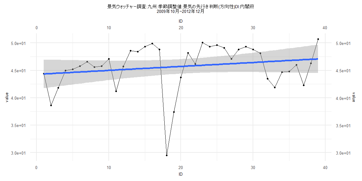
Call:
lm(formula = value ~ ID)

Residuals:
     Min       1Q   Median       3Q      Max
-16.0789  -2.0136   0.8696   2.9364   4.4652

Coefficients:
            Estimate Std. Error t value            Pr(>|t|)
(Intercept) 44.28178    1.33687  33.124 <0.0000000000000002 ***
ID           0.07206    0.05825   1.237               0.224
---
Signif. codes:  0 '***' 0.001 '**' 0.01 '*' 0.05 '.' 0.1 ' ' 1

Residual standard error: 4.094 on 37 degrees of freedom
Multiple R-squared:  0.03972,   Adjusted R-squared:  0.01377
F-statistic:  1.53 on 1 and 37 DF,  p-value: 0.2238


    Two-sample Kolmogorov-Smirnov test

data:  lm_residuals and rnorm(n = length(lm_residuals), mean = 0, sd = sd(lm_residuals))
D = 0.20513, p-value = 0.3888
alternative hypothesis: two-sided


    Durbin-Watson test

data:  value ~ ID
DW = 1.1738, p-value = 0.001836
alternative hypothesis: true autocorrelation is greater than 0


    studentized Breusch-Pagan test

data:  value ~ ID
BP = 0.012002, df = 1, p-value = 0.9128


    Box-Ljung test

data:  lm_residuals
X-squared = 6.8211, df = 1, p-value = 0.009009
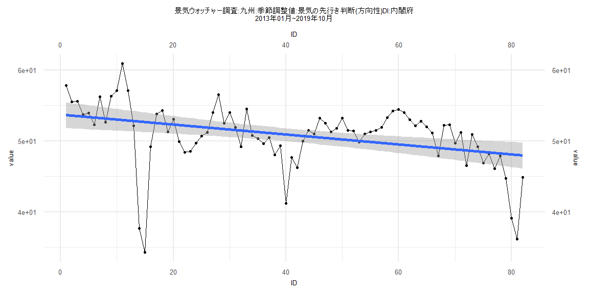
Call:
lm(formula = value ~ ID)

Residuals:
     Min       1Q   Median       3Q      Max
-18.3267  -1.4478   0.8391   2.4795   7.9930

Coefficients:
            Estimate Std. Error t value             Pr(>|t|)
(Intercept) 53.67787    0.93655  57.315 < 0.0000000000000002 ***
ID          -0.07008    0.01960  -3.575             0.000597 ***
---
Signif. codes:  0 '***' 0.001 '**' 0.01 '*' 0.05 '.' 0.1 ' ' 1

Residual standard error: 4.202 on 80 degrees of freedom
Multiple R-squared:  0.1378,    Adjusted R-squared:  0.127
F-statistic: 12.78 on 1 and 80 DF,  p-value: 0.0005975


    Two-sample Kolmogorov-Smirnov test

data:  lm_residuals and rnorm(n = length(lm_residuals), mean = 0, sd = sd(lm_residuals))
D = 0.10976, p-value = 0.7099
alternative hypothesis: two-sided


    Durbin-Watson test

data:  value ~ ID
DW = 0.75331, p-value = 0.00000000004074
alternative hypothesis: true autocorrelation is greater than 0


    studentized Breusch-Pagan test

data:  value ~ ID
BP = 0.64162, df = 1, p-value = 0.4231


    Box-Ljung test

data:  lm_residuals
X-squared = 32.045, df = 1, p-value = 0.00000001506
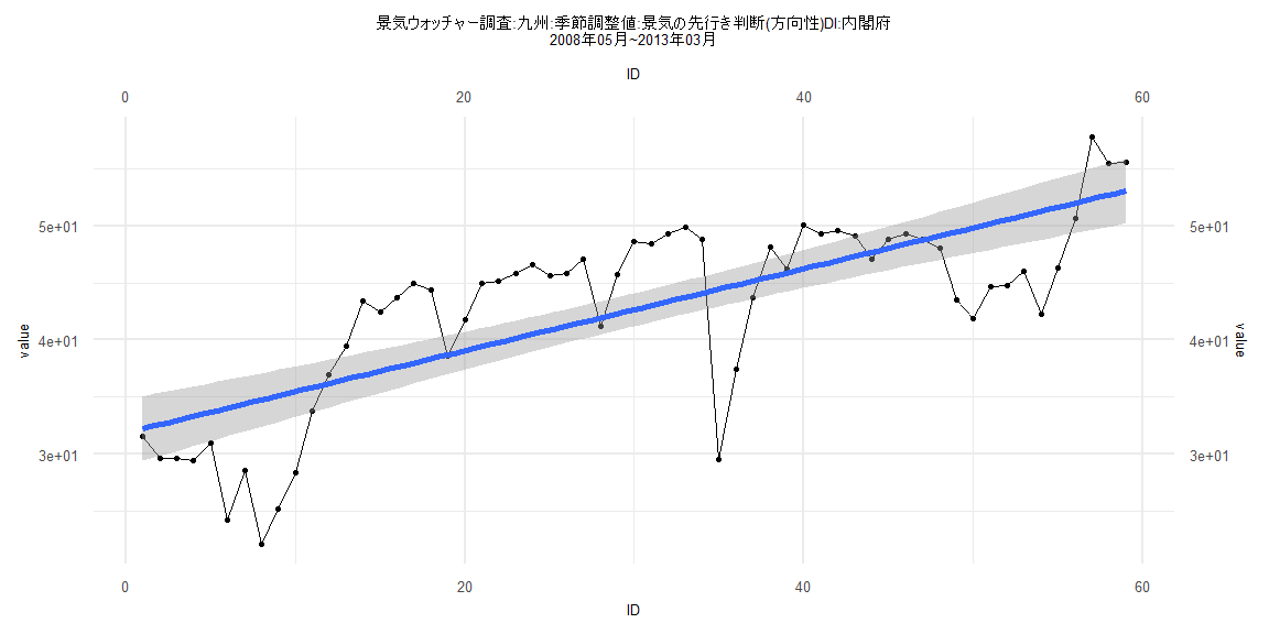
Call:
lm(formula = value ~ ID)

Residuals:
     Min       1Q   Median       3Q      Max
-14.9535  -3.6289   0.8152   4.9892   7.0177

Coefficients:
            Estimate Std. Error t value             Pr(>|t|)
(Intercept) 31.87066    1.45465  21.909 < 0.0000000000000002 ***
ID           0.35951    0.04217   8.526     0.00000000000927 ***
---
Signif. codes:  0 '***' 0.001 '**' 0.01 '*' 0.05 '.' 0.1 ' ' 1

Residual standard error: 5.516 on 57 degrees of freedom
Multiple R-squared:  0.5605,    Adjusted R-squared:  0.5528
F-statistic: 72.69 on 1 and 57 DF,  p-value: 0.000000000009274


    Two-sample Kolmogorov-Smirnov test

data:  lm_residuals and rnorm(n = length(lm_residuals), mean = 0, sd = sd(lm_residuals))
D = 0.16949, p-value = 0.3674
alternative hypothesis: two-sided


    Durbin-Watson test

data:  value ~ ID
DW = 0.56174, p-value = 0.000000000007583
alternative hypothesis: true autocorrelation is greater than 0


    studentized Breusch-Pagan test

data:  value ~ ID
BP = 1.0299, df = 1, p-value = 0.3102


    Box-Ljung test

data:  lm_residuals
X-squared = 31.917, df = 1, p-value = 0.00000001609
Call:
lm(formula = value ~ ID)

Residuals:
    Min      1Q  Median      3Q     Max
-17.989  -1.449   0.808   2.545   8.364

Coefficients:
            Estimate Std. Error t value             Pr(>|t|)
(Intercept) 53.02989    0.96264  55.088 < 0.0000000000000002 ***
ID          -0.06176    0.02091  -2.954              0.00416 **
---
Signif. codes:  0 '***' 0.001 '**' 0.01 '*' 0.05 '.' 0.1 ' ' 1

Residual standard error: 4.237 on 77 degrees of freedom
Multiple R-squared:  0.1018,    Adjusted R-squared:  0.09013
F-statistic: 8.726 on 1 and 77 DF,  p-value: 0.004159


    Two-sample Kolmogorov-Smirnov test

data:  lm_residuals and rnorm(n = length(lm_residuals), mean = 0, sd = sd(lm_residuals))
D = 0.17722, p-value = 0.1677
alternative hypothesis: two-sided


    Durbin-Watson test

data:  value ~ ID
DW = 0.76349, p-value = 0.0000000001326
alternative hypothesis: true autocorrelation is greater than 0


    studentized Breusch-Pagan test

data:  value ~ ID
BP = 0.83042, df = 1, p-value = 0.3622


    Box-Ljung test

data:  lm_residuals
X-squared = 30.952, df = 1, p-value = 0.00000002644