Analysis
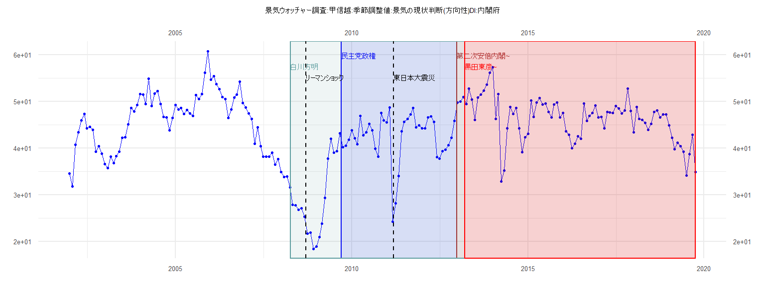
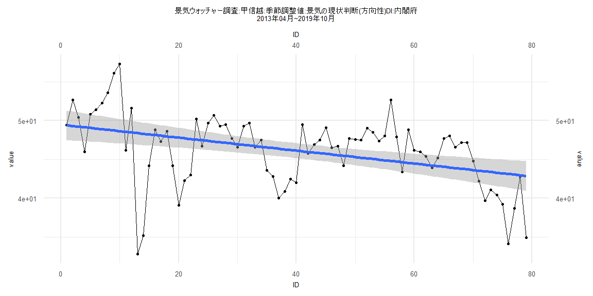
[1] "景気ウォッチャー調査:甲信越:季節調整値:景気の現状判断(方向性)DI:内閣府"
      Jan  Feb  Mar  Apr  May  Jun  Jul  Aug  Sep  Oct  Nov  Dec
2002 34.5 31.8 40.7 43.4 45.9 47.3 44.2 44.5 43.9 39.2 40.4 38.8
2003 36.6 35.7 38.1 36.8 38.3 39.2 42.2 42.3 45.1 48.6 47.8 49.2
2004 51.6 51.4 49.4 54.9 49.0 51.7 52.2 49.4 46.7 46.5 43.8 46.4
2005 49.2 48.3 48.6 47.3 48.2 47.4 46.9 51.3 50.5 51.6 56.1 60.7
2006 54.6 55.4 53.7 52.6 50.9 50.5 46.4 48.3 50.8 51.4 54.2 49.6
2007 48.7 47.4 46.2 40.9 44.4 40.4 38.1 38.1 38.1 39.0 36.4 37.6
2008 34.8 33.8 33.9 31.6 27.8 27.7 26.8 27.1 25.3 21.7 21.9 18.4
2009 18.9 20.9 23.8 29.3 37.7 42.0 39.0 39.3 43.2 40.2 40.5 41.8
2010 43.8 42.1 40.8 46.9 42.7 43.4 45.2 43.8 39.9 38.1 47.5 45.9
2011 45.5 48.7 24.2 28.1 34.0 43.6 45.6 46.2 47.2 48.6 44.4 44.8
2012 44.2 44.2 46.5 46.8 45.6 38.0 37.7 39.3 39.6 40.6 42.2 45.8
2013 49.7 50.0 50.9 49.4 52.7 50.4 46.0 50.8 51.4 52.3 53.6 56.1
2014 57.3 46.2 51.6 32.8 35.2 44.2 48.8 47.3 48.6 44.2 39.1 42.3
2015 43.0 50.2 46.7 49.7 50.7 49.3 49.5 47.7 46.6 49.3 49.7 46.6
2016 47.5 43.6 42.8 40.0 40.9 42.5 42.0 49.5 45.8 46.9 47.5 49.1
2017 46.5 46.7 44.2 47.7 47.6 47.5 49.0 48.5 47.4 48.0 52.7 47.9
2018 43.4 48.8 46.2 46.0 45.4 43.9 45.2 47.7 48.0 46.6 47.2 47.2
2019 44.8 42.2 39.7 41.1 40.4 39.2 34.1 38.7 42.8 34.9
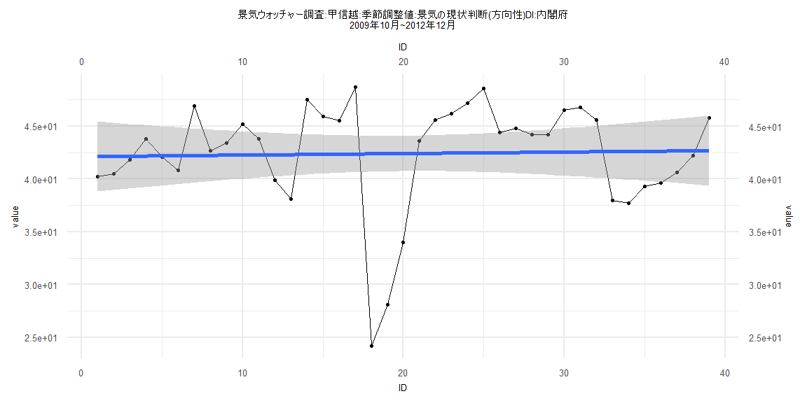
Call:
lm(formula = value ~ ID)

Residuals:
    Min      1Q  Median      3Q     Max
-18.182  -1.996   1.519   3.154   6.333

Coefficients:
            Estimate Std. Error t value            Pr(>|t|)
(Intercept) 42.12321    1.68565  24.989 <0.0000000000000002 ***
ID           0.01435    0.07345   0.195               0.846
---
Signif. codes:  0 '***' 0.001 '**' 0.01 '*' 0.05 '.' 0.1 ' ' 1

Residual standard error: 5.163 on 37 degrees of freedom
Multiple R-squared:  0.001031,  Adjusted R-squared:  -0.02597
F-statistic: 0.03818 on 1 and 37 DF,  p-value: 0.8462


    Two-sample Kolmogorov-Smirnov test

data:  lm_residuals and rnorm(n = length(lm_residuals), mean = 0, sd = sd(lm_residuals))
D = 0.25641, p-value = 0.1547
alternative hypothesis: two-sided


    Durbin-Watson test

data:  value ~ ID
DW = 1.0569, p-value = 0.0004166
alternative hypothesis: true autocorrelation is greater than 0


    studentized Breusch-Pagan test

data:  value ~ ID
BP = 0.00031105, df = 1, p-value = 0.9859


    Box-Ljung test

data:  lm_residuals
X-squared = 9.0868, df = 1, p-value = 0.002575
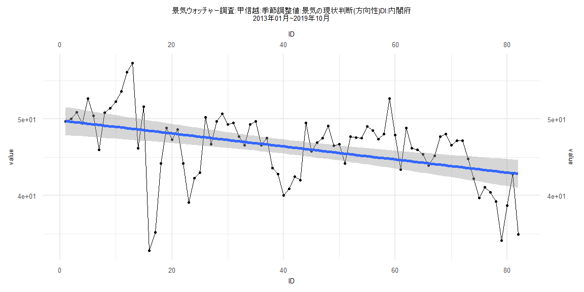
Call:
lm(formula = value ~ ID)

Residuals:
    Min      1Q  Median      3Q     Max
-15.655  -2.380   1.045   2.708   8.590

Coefficients:
            Estimate Std. Error t value             Pr(>|t|)
(Intercept) 49.81771    0.93914  53.046 < 0.0000000000000002 ***
ID          -0.08518    0.01966  -4.333            0.0000424 ***
---
Signif. codes:  0 '***' 0.001 '**' 0.01 '*' 0.05 '.' 0.1 ' ' 1

Residual standard error: 4.213 on 80 degrees of freedom
Multiple R-squared:  0.1901,    Adjusted R-squared:   0.18
F-statistic: 18.77 on 1 and 80 DF,  p-value: 0.00004237


    Two-sample Kolmogorov-Smirnov test

data:  lm_residuals and rnorm(n = length(lm_residuals), mean = 0, sd = sd(lm_residuals))
D = 0.26829, p-value = 0.005274
alternative hypothesis: two-sided


    Durbin-Watson test

data:  value ~ ID
DW = 0.87078, p-value = 0.000000004405
alternative hypothesis: true autocorrelation is greater than 0


    studentized Breusch-Pagan test

data:  value ~ ID
BP = 1.0789, df = 1, p-value = 0.2989


    Box-Ljung test

data:  lm_residuals
X-squared = 25.023, df = 1, p-value = 0.0000005666
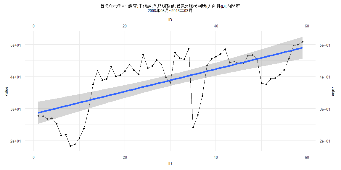
Call:
lm(formula = value ~ ID)

Residuals:
    Min      1Q  Median      3Q     Max
-16.456  -5.155   1.341   5.495  10.096

Coefficients:
            Estimate Std. Error t value             Pr(>|t|)
(Intercept) 28.40088    1.76466  16.094 < 0.0000000000000002 ***
ID           0.35014    0.05115   6.845        0.00000000577 ***
---
Signif. codes:  0 '***' 0.001 '**' 0.01 '*' 0.05 '.' 0.1 ' ' 1

Residual standard error: 6.691 on 57 degrees of freedom
Multiple R-squared:  0.4511,    Adjusted R-squared:  0.4415
F-statistic: 46.85 on 1 and 57 DF,  p-value: 0.000000005771


    Two-sample Kolmogorov-Smirnov test

data:  lm_residuals and rnorm(n = length(lm_residuals), mean = 0, sd = sd(lm_residuals))
D = 0.10169, p-value = 0.9239
alternative hypothesis: two-sided


    Durbin-Watson test

data:  value ~ ID
DW = 0.48749, p-value = 0.0000000000001734
alternative hypothesis: true autocorrelation is greater than 0


    studentized Breusch-Pagan test

data:  value ~ ID
BP = 2.6545, df = 1, p-value = 0.1033


    Box-Ljung test

data:  lm_residuals
X-squared = 35.41, df = 1, p-value = 0.000000002671
Call:
lm(formula = value ~ ID)

Residuals:
    Min      1Q  Median      3Q     Max
-15.590  -2.625   1.071   2.810   8.659

Coefficients:
            Estimate Std. Error t value             Pr(>|t|)
(Intercept) 49.47634    0.97490  50.750 < 0.0000000000000002 ***
ID          -0.08355    0.02117  -3.946             0.000174 ***
---
Signif. codes:  0 '***' 0.001 '**' 0.01 '*' 0.05 '.' 0.1 ' ' 1

Residual standard error: 4.291 on 77 degrees of freedom
Multiple R-squared:  0.1682,    Adjusted R-squared:  0.1574
F-statistic: 15.57 on 1 and 77 DF,  p-value: 0.0001741


    Two-sample Kolmogorov-Smirnov test

data:  lm_residuals and rnorm(n = length(lm_residuals), mean = 0, sd = sd(lm_residuals))
D = 0.13924, p-value = 0.4302
alternative hypothesis: two-sided


    Durbin-Watson test

data:  value ~ ID
DW = 0.86986, p-value = 0.000000007696
alternative hypothesis: true autocorrelation is greater than 0


    studentized Breusch-Pagan test

data:  value ~ ID
BP = 1.8577, df = 1, p-value = 0.1729


    Box-Ljung test

data:  lm_residuals
X-squared = 24.157, df = 1, p-value = 0.0000008878