Analysis
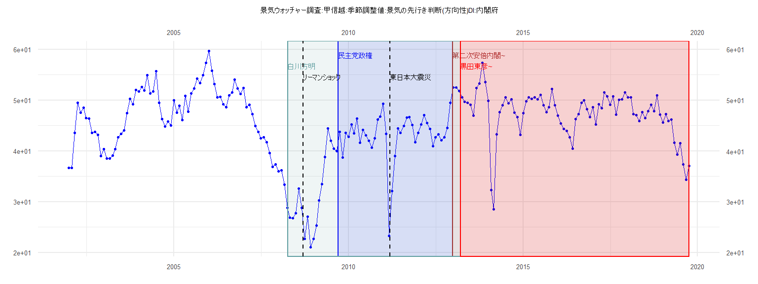
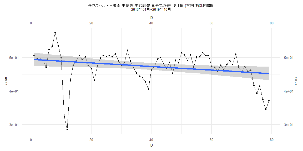
[1] "景気ウォッチャー調査:甲信越:季節調整値:景気の先行き判断(方向性)DI:内閣府"
      Jan  Feb  Mar  Apr  May  Jun  Jul  Aug  Sep  Oct  Nov  Dec
2002 36.7 36.7 43.6 49.5 47.6 48.5 46.5 46.4 43.6 43.8 43.2 39.0
2003 40.4 38.5 38.5 39.1 40.4 42.7 43.4 44.1 47.5 50.3 49.2 52.0
2004 51.7 52.6 51.9 54.9 51.4 51.7 55.7 49.5 46.3 44.8 45.8 45.0
2005 50.0 47.6 48.9 46.1 50.9 47.8 51.4 52.3 54.3 53.4 54.9 57.4
2006 59.7 55.8 53.2 50.6 50.7 49.2 48.6 51.0 51.5 54.1 52.3 51.3
2007 52.4 48.6 49.1 47.3 44.9 43.8 42.5 42.7 41.7 39.6 36.9 37.4
2008 36.0 36.2 33.4 28.8 26.9 26.8 27.8 32.6 28.8 22.7 27.1 21.1
2009 22.7 25.3 30.3 33.5 38.8 44.5 42.0 40.5 40.0 43.8 38.7 43.6
2010 42.8 45.2 43.5 46.4 41.6 44.2 43.1 42.0 40.7 42.5 46.2 46.8
2011 49.3 43.4 23.3 32.1 39.0 44.5 43.6 44.9 46.6 46.7 45.1 41.7
2012 43.6 45.2 47.1 45.5 44.4 41.0 42.7 43.3 42.1 42.7 44.6 49.5
2013 52.5 52.5 51.8 50.6 49.7 49.5 49.1 47.0 52.4 53.3 57.4 53.6
2014 49.9 32.3 28.5 43.3 47.7 49.0 50.6 49.4 50.2 47.6 46.7 43.2
2015 47.5 49.8 50.6 50.3 50.6 50.2 51.1 49.0 47.7 48.6 52.2 49.0
2016 47.0 45.4 44.4 44.0 42.7 40.5 46.3 47.3 49.5 50.0 48.2 46.7
2017 48.6 45.2 49.2 48.4 51.5 50.8 49.1 50.8 47.2 50.1 50.2 51.5
2018 50.6 50.6 47.3 47.1 45.9 47.7 46.5 47.9 49.1 47.9 51.0 47.2
2019 45.6 47.3 45.9 46.2 41.6 39.3 41.5 37.4 34.4 37.1
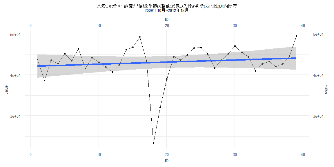
Call:
lm(formula = value ~ ID)

Residuals:
     Min       1Q   Median       3Q      Max
-19.7518  -1.0549   0.5279   1.7126   6.3502

Coefficients:
            Estimate Std. Error t value            Pr(>|t|)
(Intercept) 42.13360    1.45910  28.876 <0.0000000000000002 ***
ID           0.05101    0.06358   0.802               0.427
---
Signif. codes:  0 '***' 0.001 '**' 0.01 '*' 0.05 '.' 0.1 ' ' 1

Residual standard error: 4.469 on 37 degrees of freedom
Multiple R-squared:  0.0171,    Adjusted R-squared:  -0.009464
F-statistic: 0.6437 on 1 and 37 DF,  p-value: 0.4275


    Two-sample Kolmogorov-Smirnov test

data:  lm_residuals and rnorm(n = length(lm_residuals), mean = 0, sd = sd(lm_residuals))
D = 0.17949, p-value = 0.5622
alternative hypothesis: two-sided


    Durbin-Watson test

data:  value ~ ID
DW = 1.0775, p-value = 0.0005509
alternative hypothesis: true autocorrelation is greater than 0


    studentized Breusch-Pagan test

data:  value ~ ID
BP = 0.034911, df = 1, p-value = 0.8518


    Box-Ljung test

data:  lm_residuals
X-squared = 8.1439, df = 1, p-value = 0.004321
Call:
lm(formula = value ~ ID)

Residuals:
     Min       1Q   Median       3Q      Max
-20.5978  -1.0523   0.9556   2.3360   8.0593

Coefficients:
            Estimate Std. Error t value            Pr(>|t|)
(Intercept) 50.00849    0.99969  50.024 <0.0000000000000002 ***
ID          -0.06071    0.02092  -2.901              0.0048 **
---
Signif. codes:  0 '***' 0.001 '**' 0.01 '*' 0.05 '.' 0.1 ' ' 1

Residual standard error: 4.485 on 80 degrees of freedom
Multiple R-squared:  0.09521,   Adjusted R-squared:  0.0839
F-statistic: 8.418 on 1 and 80 DF,  p-value: 0.004797


    Two-sample Kolmogorov-Smirnov test

data:  lm_residuals and rnorm(n = length(lm_residuals), mean = 0, sd = sd(lm_residuals))
D = 0.2439, p-value = 0.01494
alternative hypothesis: two-sided


    Durbin-Watson test

data:  value ~ ID
DW = 0.60527, p-value = 0.00000000000002259
alternative hypothesis: true autocorrelation is greater than 0


    studentized Breusch-Pagan test

data:  value ~ ID
BP = 0.59109, df = 1, p-value = 0.442


    Box-Ljung test

data:  lm_residuals
X-squared = 38.837, df = 1, p-value = 0.0000000004607
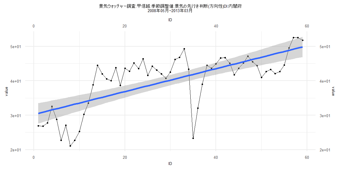
Call:
lm(formula = value ~ ID)

Residuals:
    Min      1Q  Median      3Q     Max
-18.553  -3.606   1.059   4.021   9.633

Coefficients:
            Estimate Std. Error t value             Pr(>|t|)
(Intercept)  30.2102     1.5111  19.992 < 0.0000000000000002 ***
ID            0.3327     0.0438   7.594       0.000000000325 ***
---
Signif. codes:  0 '***' 0.001 '**' 0.01 '*' 0.05 '.' 0.1 ' ' 1

Residual standard error: 5.73 on 57 degrees of freedom
Multiple R-squared:  0.5029,    Adjusted R-squared:  0.4942
F-statistic: 57.67 on 1 and 57 DF,  p-value: 0.0000000003254


    Two-sample Kolmogorov-Smirnov test

data:  lm_residuals and rnorm(n = length(lm_residuals), mean = 0, sd = sd(lm_residuals))
D = 0.22034, p-value = 0.1141
alternative hypothesis: two-sided


    Durbin-Watson test

data:  value ~ ID
DW = 0.56394, p-value = 0.000000000008403
alternative hypothesis: true autocorrelation is greater than 0


    studentized Breusch-Pagan test

data:  value ~ ID
BP = 2.1523, df = 1, p-value = 0.1424


    Box-Ljung test

data:  lm_residuals
X-squared = 31.586, df = 1, p-value = 0.00000001908
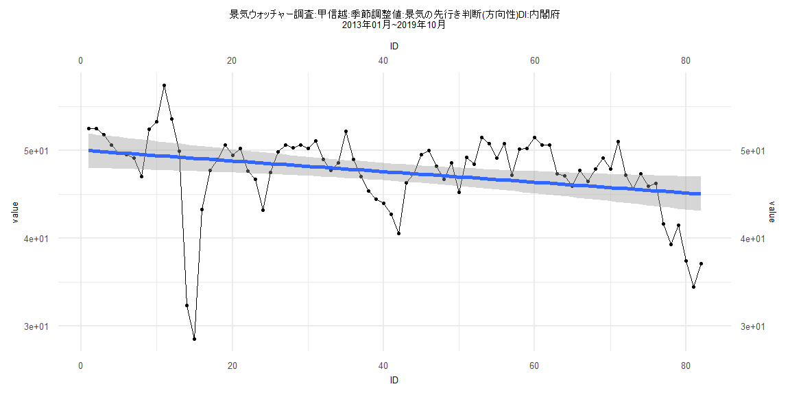
Call:
lm(formula = value ~ ID)

Residuals:
     Min       1Q   Median       3Q      Max
-20.3076  -0.9165   0.9853   2.3781   8.3781

Coefficients:
            Estimate Std. Error t value            Pr(>|t|)
(Intercept) 49.45044    1.03204   47.91 <0.0000000000000002 ***
ID          -0.05357    0.02241   -2.39              0.0193 *
---
Signif. codes:  0 '***' 0.001 '**' 0.01 '*' 0.05 '.' 0.1 ' ' 1

Residual standard error: 4.543 on 77 degrees of freedom
Multiple R-squared:  0.06906,   Adjusted R-squared:  0.05697
F-statistic: 5.712 on 1 and 77 DF,  p-value: 0.01929


    Two-sample Kolmogorov-Smirnov test

data:  lm_residuals and rnorm(n = length(lm_residuals), mean = 0, sd = sd(lm_residuals))
D = 0.17722, p-value = 0.1677
alternative hypothesis: two-sided


    Durbin-Watson test

data:  value ~ ID
DW = 0.61188, p-value = 0.0000000000000899
alternative hypothesis: true autocorrelation is greater than 0


    studentized Breusch-Pagan test

data:  value ~ ID
BP = 0.82946, df = 1, p-value = 0.3624


    Box-Ljung test

data:  lm_residuals
X-squared = 37.143, df = 1, p-value = 0.000000001098