Analysis
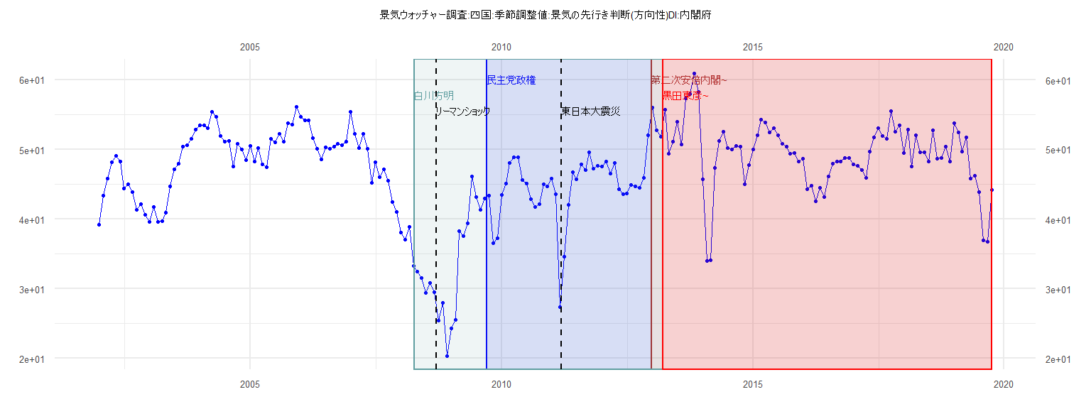
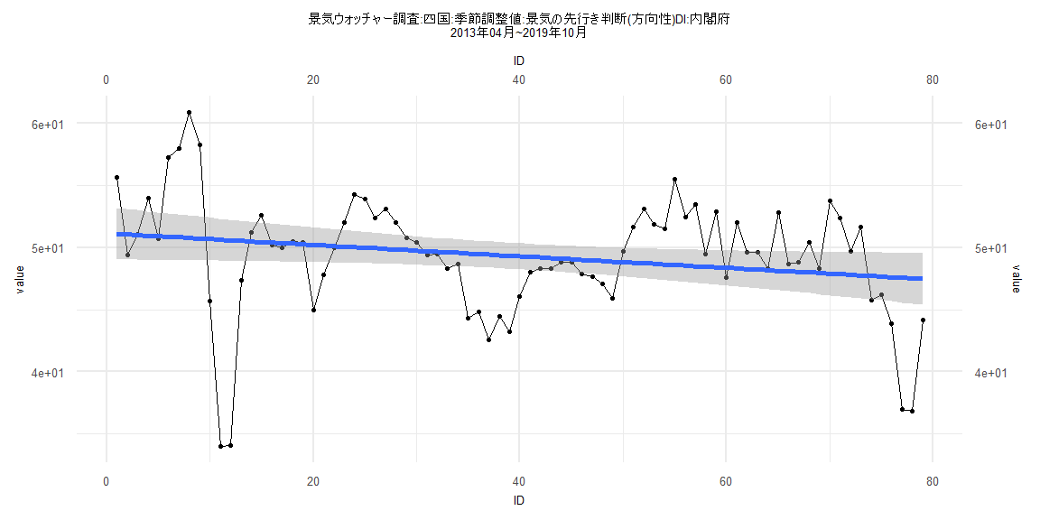
[1] "景気ウォッチャー調査:四国:季節調整値:景気の先行き判断(方向性)DI:内閣府"
Jan Feb Mar Apr May Jun Jul Aug Sep Oct Nov Dec
2002 39.2 43.4 45.8 48.2 49.1 48.3 44.4 45.0 43.9 41.3 42.2 40.6
2003 39.6 41.8 39.6 39.7 40.9 44.7 47.2 48.0 50.4 50.6 51.5 52.9
2004 53.5 53.5 53.1 55.4 54.7 51.9 51.1 51.2 47.6 50.8 50.0 48.5
2005 50.5 48.3 50.2 47.9 47.5 51.5 51.0 52.2 51.1 53.8 53.6 56.1
2006 54.7 54.2 54.2 51.6 50.1 48.6 50.3 50.1 50.4 50.8 50.6 51.1
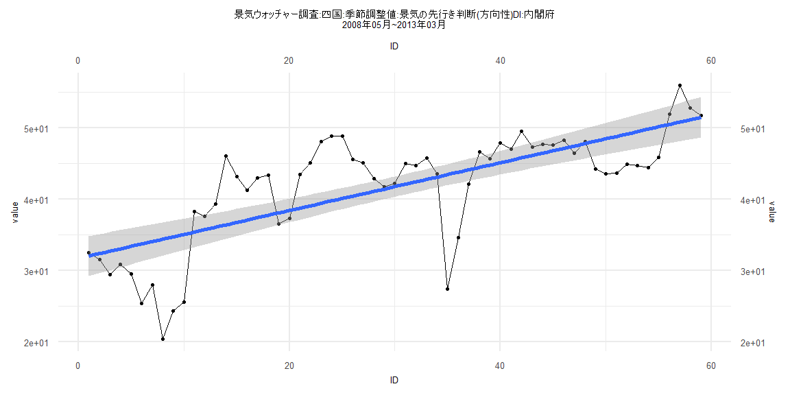
2007 55.4 52.2 50.2 52.2 50.1 45.2 48.2 46.0 47.2 45.5 42.5 41.0
2008 38.1 37.1 38.9 33.3 32.5 31.6 29.4 30.9 29.5 25.4 28.0 20.4
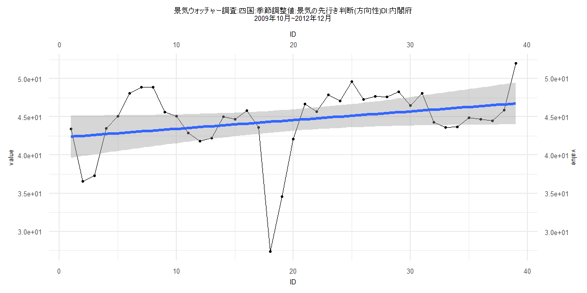
2009 24.3 25.6 38.3 37.6 39.4 46.1 43.2 41.3 43.0 43.4 36.6 37.3
2010 43.5 45.1 48.1 48.9 48.9 45.6 45.1 42.9 41.8 42.2 45.0 44.7
2011 45.8 43.6 27.4 34.6 42.1 46.7 45.7 47.9 47.1 49.6 47.3 47.7
2012 47.6 48.3 46.5 48.1 44.3 43.6 43.7 44.9 44.7 44.5 45.9 52.0
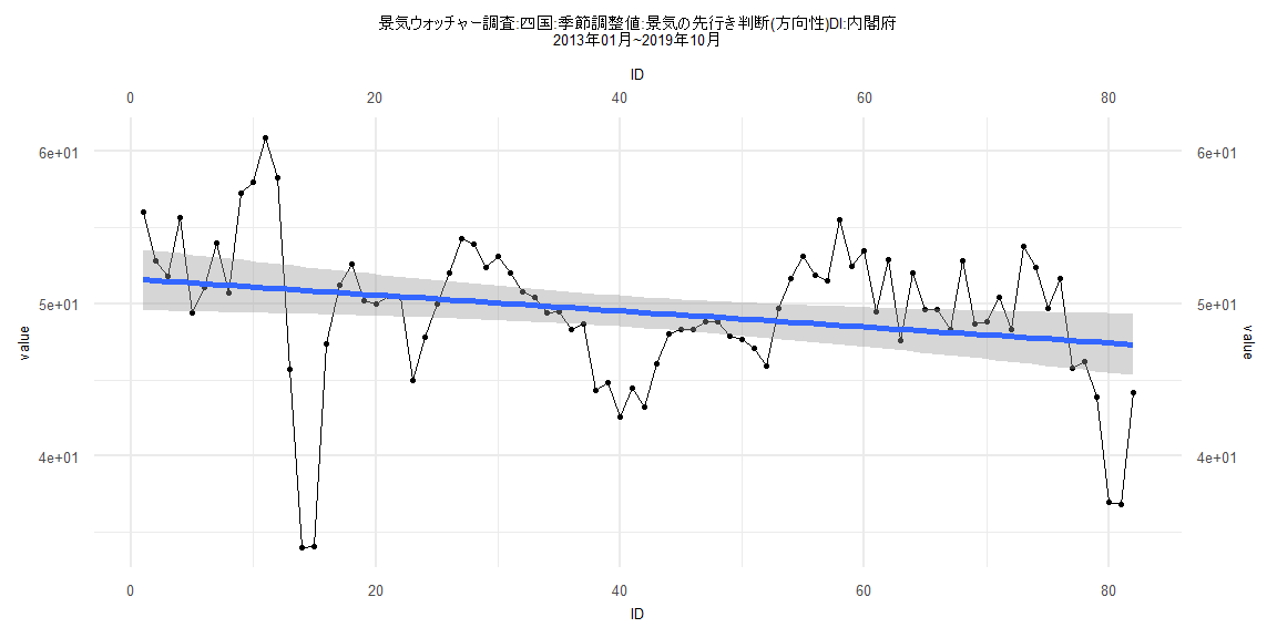
2013 56.0 52.8 51.8 55.7 49.4 51.1 54.0 50.7 57.3 58.0 60.9 58.3
2014 45.7 34.0 34.1 47.4 51.2 52.6 50.2 50.0 50.5 50.4 45.0 47.8
2015 50.0 52.0 54.3 53.9 52.4 53.1 52.0 50.8 50.4 49.4 49.5 48.3
2016 48.7 44.3 44.8 42.6 44.5 43.2 46.1 48.0 48.3 48.3 48.8 48.8
2017 47.9 47.7 47.1 45.9 49.7 51.7 53.1 51.9 51.5 55.5 52.5 53.5
2018 49.5 52.9 47.6 52.0 49.6 49.6 48.3 52.8 48.7 48.8 50.4 48.3
2019 53.8 52.4 49.7 51.7 45.8 46.2 43.9 37.0 36.8 44.2
Call:
lm(formula = value ~ ID)

Residuals:
     Min       1Q   Median       3Q      Max
-16.9538  -1.6799   0.8897   2.2462   5.8016

Coefficients:
            Estimate Std. Error t value            Pr(>|t|)
(Intercept)  42.2995     1.4092  30.017 <0.0000000000000002 ***
ID            0.1141     0.0614   1.859               0.071 .
---
Signif. codes:  0 '***' 0.001 '**' 0.01 '*' 0.05 '.' 0.1 ' ' 1

Residual standard error: 4.316 on 37 degrees of freedom
Multiple R-squared:  0.08539,   Adjusted R-squared:  0.06068
F-statistic: 3.455 on 1 and 37 DF,  p-value: 0.07104


    Two-sample Kolmogorov-Smirnov test

data:  lm_residuals and rnorm(n = length(lm_residuals), mean = 0, sd = sd(lm_residuals))
D = 0.28205, p-value = 0.08974
alternative hypothesis: two-sided


    Durbin-Watson test

data:  value ~ ID
DW = 0.86921, p-value = 0.00002083
alternative hypothesis: true autocorrelation is greater than 0


    studentized Breusch-Pagan test

data:  value ~ ID
BP = 0.36141, df = 1, p-value = 0.5477


    Box-Ljung test

data:  lm_residuals
X-squared = 12.485, df = 1, p-value = 0.0004103
Call:
lm(formula = value ~ ID)

Residuals:
     Min       1Q   Median       3Q      Max
-16.8977  -1.4190   0.2532   2.8885   9.8450

Coefficients:
            Estimate Std. Error t value            Pr(>|t|)
(Intercept) 51.63162    1.03158  50.051 <0.0000000000000002 ***
ID          -0.05242    0.02159  -2.428              0.0174 *
---
Signif. codes:  0 '***' 0.001 '**' 0.01 '*' 0.05 '.' 0.1 ' ' 1

Residual standard error: 4.628 on 80 degrees of freedom
Multiple R-squared:  0.06862,   Adjusted R-squared:  0.05698
F-statistic: 5.894 on 1 and 80 DF,  p-value: 0.01743


    Two-sample Kolmogorov-Smirnov test

data:  lm_residuals and rnorm(n = length(lm_residuals), mean = 0, sd = sd(lm_residuals))
D = 0.23171, p-value = 0.02418
alternative hypothesis: two-sided


    Durbin-Watson test

data:  value ~ ID
DW = 0.64571, p-value = 0.0000000000002171
alternative hypothesis: true autocorrelation is greater than 0


    studentized Breusch-Pagan test

data:  value ~ ID
BP = 1.1982, df = 1, p-value = 0.2737


    Box-Ljung test

data:  lm_residuals
X-squared = 38.011, df = 1, p-value = 0.0000000007034
Call:
lm(formula = value ~ ID)

Residuals:
     Min       1Q   Median       3Q      Max
-16.0716  -3.6005   0.8857   3.1565   9.6777

Coefficients:
            Estimate Std. Error t value             Pr(>|t|)
(Intercept) 31.72279    1.44373  21.973 < 0.0000000000000002 ***
ID           0.33568    0.04185   8.021      0.0000000000635 ***
---
Signif. codes:  0 '***' 0.001 '**' 0.01 '*' 0.05 '.' 0.1 ' ' 1

Residual standard error: 5.474 on 57 degrees of freedom
Multiple R-squared:  0.5302,    Adjusted R-squared:  0.522
F-statistic: 64.33 on 1 and 57 DF,  p-value: 0.00000000006349


    Two-sample Kolmogorov-Smirnov test

data:  lm_residuals and rnorm(n = length(lm_residuals), mean = 0, sd = sd(lm_residuals))
D = 0.28814, p-value = 0.01452
alternative hypothesis: two-sided


    Durbin-Watson test

data:  value ~ ID
DW = 0.55869, p-value = 0.000000000006573
alternative hypothesis: true autocorrelation is greater than 0


    studentized Breusch-Pagan test

data:  value ~ ID
BP = 3.1741, df = 1, p-value = 0.07481


    Box-Ljung test

data:  lm_residuals
X-squared = 32.219, df = 1, p-value = 0.00000001377
Call:
lm(formula = value ~ ID)

Residuals:
     Min       1Q   Median       3Q      Max
-16.6444  -1.5707   0.1261   2.9698  10.1167

Coefficients:
            Estimate Std. Error t value            Pr(>|t|)
(Intercept) 51.15385    1.06434  48.062 <0.0000000000000002 ***
ID          -0.04631    0.02312  -2.004              0.0486 *
---
Signif. codes:  0 '***' 0.001 '**' 0.01 '*' 0.05 '.' 0.1 ' ' 1

Residual standard error: 4.685 on 77 degrees of freedom
Multiple R-squared:  0.04955,   Adjusted R-squared:  0.03721
F-statistic: 4.014 on 1 and 77 DF,  p-value: 0.04863


    Two-sample Kolmogorov-Smirnov test

data:  lm_residuals and rnorm(n = length(lm_residuals), mean = 0, sd = sd(lm_residuals))
D = 0.13924, p-value = 0.4302
alternative hypothesis: two-sided


    Durbin-Watson test

data:  value ~ ID
DW = 0.63902, p-value = 0.0000000000003891
alternative hypothesis: true autocorrelation is greater than 0


    studentized Breusch-Pagan test

data:  value ~ ID
BP = 1.7662, df = 1, p-value = 0.1839


    Box-Ljung test

data:  lm_residuals
X-squared = 36.941, df = 1, p-value = 0.000000001217