Analysis
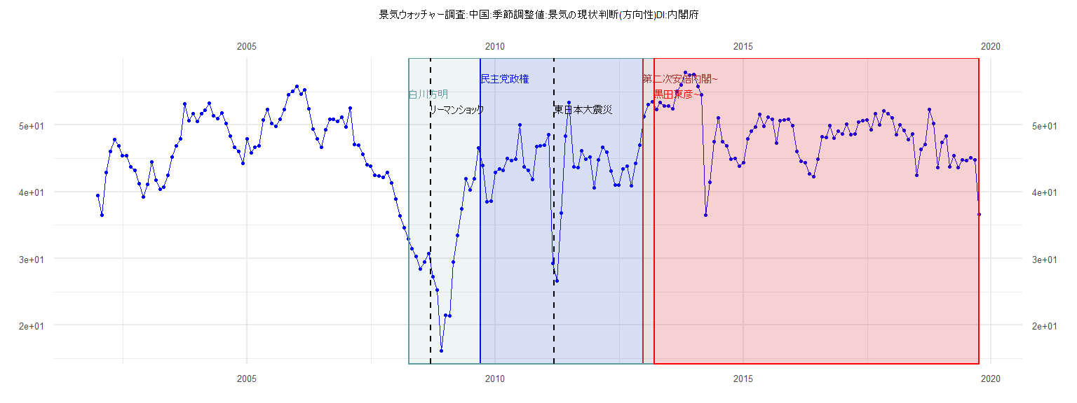
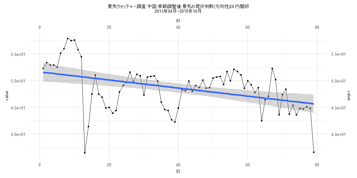
[1] "景気ウォッチャー調査:中国:季節調整値:景気の現状判断(方向性)DI:内閣府"
      Jan  Feb  Mar  Apr  May  Jun  Jul  Aug  Sep  Oct  Nov  Dec
2002 39.4 36.5 42.9 46.0 47.8 46.9 45.4 45.4 43.7 43.2 41.2 39.2
2003 41.1 44.5 41.8 40.4 40.7 42.5 45.2 46.9 47.9 53.2 50.7 51.7
2004 50.6 51.7 52.2 53.3 51.4 51.0 51.8 50.2 48.4 46.7 46.1 44.3
2005 47.9 45.8 46.7 46.9 50.8 52.3 50.2 49.8 50.9 52.3 54.5 55.1
2006 55.8 54.7 55.3 52.5 49.4 47.9 46.7 49.3 50.9 50.9 50.6 51.2
2007 49.7 52.6 47.1 47.0 45.6 44.1 43.8 42.5 42.4 42.2 42.9 41.3
2008 38.9 36.4 34.6 32.9 31.5 30.3 28.4 29.5 30.7 27.3 25.3 16.2
2009 21.5 21.4 29.5 33.5 37.5 42.0 40.3 42.0 46.6 44.0 38.5 38.6
2010 42.9 43.4 43.2 45.0 44.7 44.9 50.0 43.7 43.2 41.9 46.8 46.9
2011 47.0 48.6 29.3 26.6 36.8 48.4 53.4 43.7 43.6 46.2 44.9 45.2
2012 40.6 44.8 46.7 45.9 43.1 41.0 41.0 43.4 43.9 40.9 44.3 47.0
2013 51.3 53.1 53.5 52.3 53.4 52.9 52.9 52.5 55.1 56.0 57.9 57.5
2014 57.6 55.8 54.5 36.5 41.4 47.5 51.1 47.5 46.9 44.9 45.0 43.9
2015 44.4 47.9 49.1 49.7 51.6 49.8 51.2 50.9 47.3 50.7 50.8 50.9
2016 49.9 46.0 44.6 44.4 42.7 42.3 44.9 48.3 48.1 49.9 48.0 49.1
2017 48.7 50.1 48.6 48.7 50.5 50.7 50.8 49.3 51.7 50.0 52.1 51.7
2018 51.1 48.6 50.0 49.2 47.8 48.7 42.5 46.4 47.1 52.3 50.2 43.6
2019 47.4 48.4 43.7 45.4 43.6 44.8 44.7 45.1 44.8 36.6
Call:
lm(formula = value ~ ID)

Residuals:
    Min      1Q  Median      3Q     Max
-16.809  -1.002   0.385   2.401   9.911

Coefficients:
            Estimate Std. Error t value            Pr(>|t|)
(Intercept) 42.90351    1.59444  26.908 <0.0000000000000002 ***
ID           0.02662    0.06948   0.383               0.704
---
Signif. codes:  0 '***' 0.001 '**' 0.01 '*' 0.05 '.' 0.1 ' ' 1

Residual standard error: 4.883 on 37 degrees of freedom
Multiple R-squared:  0.003952,  Adjusted R-squared:  -0.02297
F-statistic: 0.1468 on 1 and 37 DF,  p-value: 0.7038


    Two-sample Kolmogorov-Smirnov test

data:  lm_residuals and rnorm(n = length(lm_residuals), mean = 0, sd = sd(lm_residuals))
D = 0.28205, p-value = 0.08974
alternative hypothesis: two-sided


    Durbin-Watson test

data:  value ~ ID
DW = 1.1127, p-value = 0.0008722
alternative hypothesis: true autocorrelation is greater than 0


    studentized Breusch-Pagan test

data:  value ~ ID
BP = 0.096933, df = 1, p-value = 0.7555


    Box-Ljung test

data:  lm_residuals
X-squared = 8.0623, df = 1, p-value = 0.00452
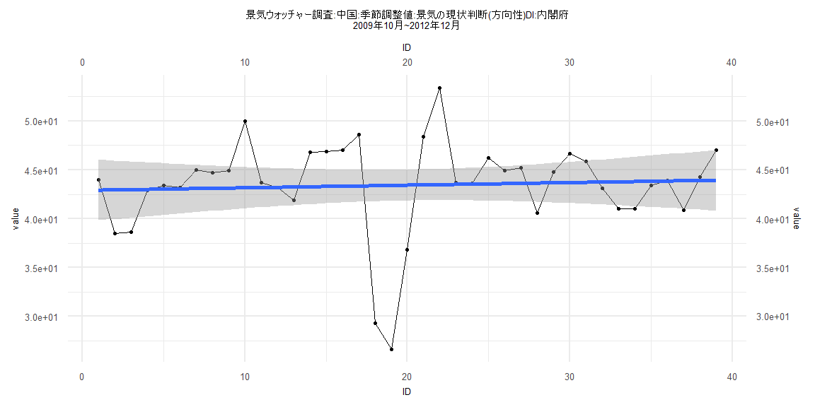
Call:
lm(formula = value ~ ID)

Residuals:
     Min       1Q   Median       3Q      Max
-14.2506  -2.1107   0.7731   1.9676   6.7593

Coefficients:
            Estimate Std. Error t value             Pr(>|t|)
(Intercept) 51.99901    0.84279  61.699 < 0.0000000000000002 ***
ID          -0.07802    0.01764  -4.423            0.0000304 ***
---
Signif. codes:  0 '***' 0.001 '**' 0.01 '*' 0.05 '.' 0.1 ' ' 1

Residual standard error: 3.781 on 80 degrees of freedom
Multiple R-squared:  0.1965,    Adjusted R-squared:  0.1864
F-statistic: 19.56 on 1 and 80 DF,  p-value: 0.00003037


    Two-sample Kolmogorov-Smirnov test

data:  lm_residuals and rnorm(n = length(lm_residuals), mean = 0, sd = sd(lm_residuals))
D = 0.19512, p-value = 0.08807
alternative hypothesis: two-sided


    Durbin-Watson test

data:  value ~ ID
DW = 0.70819, p-value = 0.000000000005143
alternative hypothesis: true autocorrelation is greater than 0


    studentized Breusch-Pagan test

data:  value ~ ID
BP = 2.3427, df = 1, p-value = 0.1259


    Box-Ljung test

data:  lm_residuals
X-squared = 31.675, df = 1, p-value = 0.00000001822
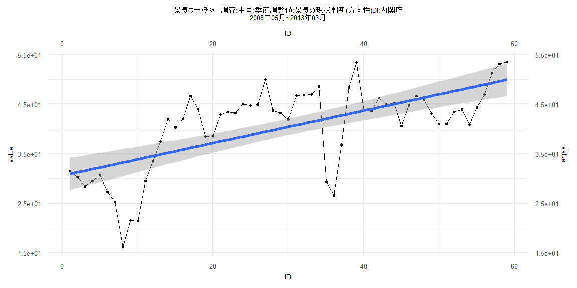
Call:
lm(formula = value ~ ID)

Residuals:
     Min       1Q   Median       3Q      Max
-17.0231  -4.1517   0.5702   5.3833  10.5523

Coefficients:
            Estimate Std. Error t value             Pr(>|t|)
(Intercept) 30.60222    1.68268  18.187 < 0.0000000000000002 ***
ID           0.32761    0.04878   6.716        0.00000000944 ***
---
Signif. codes:  0 '***' 0.001 '**' 0.01 '*' 0.05 '.' 0.1 ' ' 1

Residual standard error: 6.38 on 57 degrees of freedom
Multiple R-squared:  0.4418,    Adjusted R-squared:  0.432
F-statistic: 45.11 on 1 and 57 DF,  p-value: 0.000000009437


    Two-sample Kolmogorov-Smirnov test

data:  lm_residuals and rnorm(n = length(lm_residuals), mean = 0, sd = sd(lm_residuals))
D = 0.15254, p-value = 0.5021
alternative hypothesis: two-sided


    Durbin-Watson test

data:  value ~ ID
DW = 0.55214, p-value = 0.000000000004818
alternative hypothesis: true autocorrelation is greater than 0


    studentized Breusch-Pagan test

data:  value ~ ID
BP = 2.2293, df = 1, p-value = 0.1354


    Box-Ljung test

data:  lm_residuals
X-squared = 32.267, df = 1, p-value = 0.00000001344
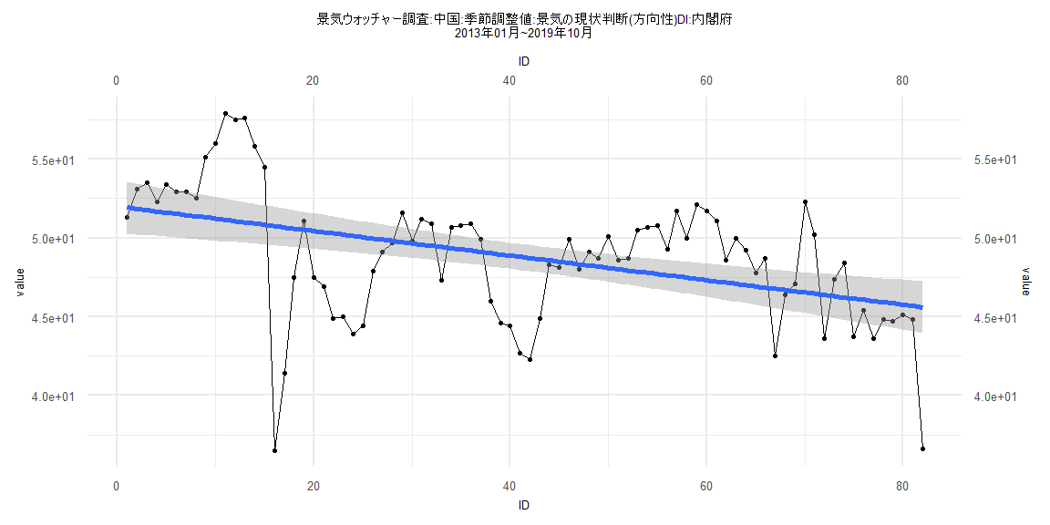
Call:
lm(formula = value ~ ID)

Residuals:
     Min       1Q   Median       3Q      Max
-14.1582  -2.2553   0.7675   2.0747   6.8632

Coefficients:
            Estimate Std. Error t value             Pr(>|t|)
(Intercept) 51.64255    0.87349  59.122 < 0.0000000000000002 ***
ID          -0.07572    0.01897  -3.991             0.000149 ***
---
Signif. codes:  0 '***' 0.001 '**' 0.01 '*' 0.05 '.' 0.1 ' ' 1

Residual standard error: 3.845 on 77 degrees of freedom
Multiple R-squared:  0.1714,    Adjusted R-squared:  0.1606
F-statistic: 15.93 on 1 and 77 DF,  p-value: 0.0001489


    Two-sample Kolmogorov-Smirnov test

data:  lm_residuals and rnorm(n = length(lm_residuals), mean = 0, sd = sd(lm_residuals))
D = 0.16456, p-value = 0.2361
alternative hypothesis: two-sided


    Durbin-Watson test

data:  value ~ ID
DW = 0.7071, p-value = 0.00000000001114
alternative hypothesis: true autocorrelation is greater than 0


    studentized Breusch-Pagan test

data:  value ~ ID
BP = 3.5794, df = 1, p-value = 0.0585


    Box-Ljung test

data:  lm_residuals
X-squared = 30.542, df = 1, p-value = 0.00000003267