Analysis
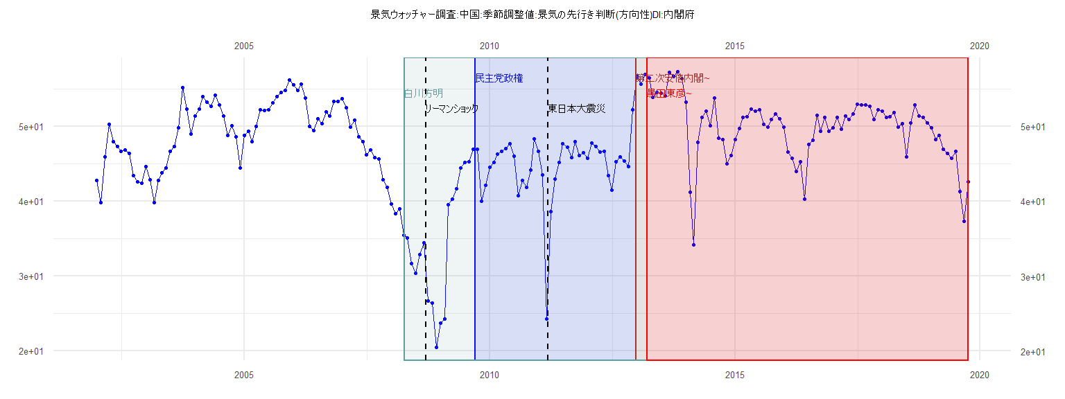
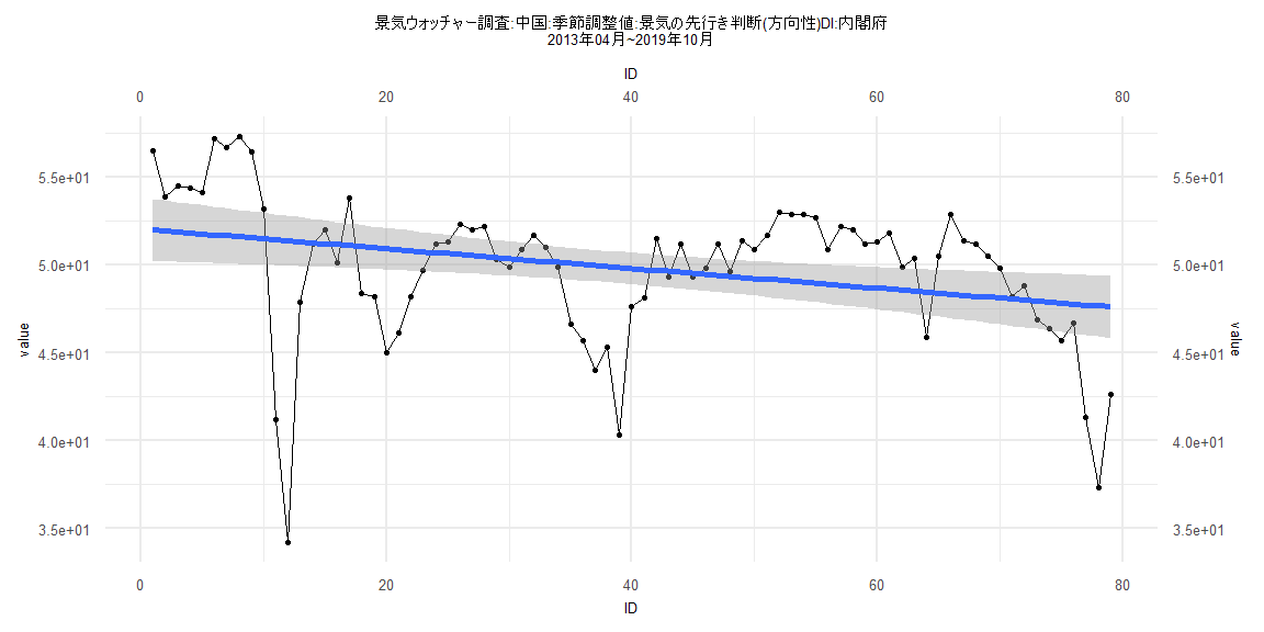
[1] "景気ウォッチャー調査:中国:季節調整値:景気の先行き判断(方向性)DI:内閣府"
      Jan  Feb  Mar  Apr  May  Jun  Jul  Aug  Sep  Oct  Nov  Dec
2002 42.8 39.8 45.9 50.3 48.0 47.3 46.7 46.8 46.4 43.4 42.6 42.4
2003 44.6 42.9 39.8 42.8 43.8 44.4 46.7 47.3 49.8 55.2 52.3 49.0
2004 51.4 52.3 54.0 53.2 52.7 54.2 52.9 51.4 48.8 50.1 48.6 44.4
2005 48.8 49.3 48.0 50.0 52.2 52.1 52.2 53.1 54.0 54.5 54.8 56.2
2006 55.5 54.8 55.6 53.8 50.0 49.4 51.0 50.4 51.9 51.4 53.3 53.3
2007 53.7 52.5 49.9 50.8 48.6 48.0 46.2 46.8 45.8 45.6 42.9 41.8
2008 39.6 38.3 39.0 35.5 35.1 31.7 30.4 32.9 34.4 26.7 26.4 20.5
2009 23.7 24.3 39.5 40.3 41.7 44.4 45.2 45.3 46.9 46.9 40.0 42.1
2010 44.5 45.2 46.3 46.7 47.0 47.7 46.0 40.7 42.8 41.8 44.2 48.3
2011 46.7 43.5 24.3 38.6 43.0 45.2 47.7 47.2 45.8 48.0 46.1 46.5
2012 45.7 47.8 47.3 46.6 46.7 43.4 41.5 45.3 45.9 45.4 44.6 52.2
2013 56.7 55.6 56.9 56.5 53.9 54.5 54.4 54.1 57.2 56.7 57.3 56.4
2014 53.2 41.2 34.2 47.9 51.2 52.0 50.1 53.8 48.4 48.2 45.0 46.1
2015 48.2 49.7 51.2 51.3 52.3 52.0 52.2 50.3 49.9 50.9 51.7 51.0
2016 49.9 46.6 45.7 44.0 45.3 40.3 47.6 48.1 51.5 49.3 51.2 49.3
2017 49.8 51.2 49.6 51.4 50.9 51.7 53.0 52.9 52.9 52.7 50.9 52.2
2018 52.0 51.2 51.3 51.8 49.9 50.4 45.9 50.5 52.9 51.4 51.2 50.5
2019 49.8 48.2 48.8 46.9 46.4 45.7 46.7 41.3 37.3 42.6
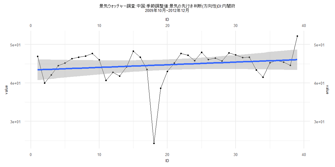
Call:
lm(formula = value ~ ID)

Residuals:
     Min       1Q   Median       3Q      Max
-20.3105  -1.3944   0.8574   2.3365   6.1378

Coefficients:
            Estimate Std. Error t value            Pr(>|t|)
(Intercept) 43.36613    1.38322  31.352 <0.0000000000000002 ***
ID           0.06913    0.06027   1.147               0.259
---
Signif. codes:  0 '***' 0.001 '**' 0.01 '*' 0.05 '.' 0.1 ' ' 1

Residual standard error: 4.236 on 37 degrees of freedom
Multiple R-squared:  0.03433,   Adjusted R-squared:  0.008234
F-statistic: 1.315 on 1 and 37 DF,  p-value: 0.2588


    Two-sample Kolmogorov-Smirnov test

data:  lm_residuals and rnorm(n = length(lm_residuals), mean = 0, sd = sd(lm_residuals))
D = 0.17949, p-value = 0.5622
alternative hypothesis: two-sided


    Durbin-Watson test

data:  value ~ ID
DW = 1.2644, p-value = 0.004941
alternative hypothesis: true autocorrelation is greater than 0


    studentized Breusch-Pagan test

data:  value ~ ID
BP = 0.036637, df = 1, p-value = 0.8482


    Box-Ljung test

data:  lm_residuals
X-squared = 4.5932, df = 1, p-value = 0.0321
Call:
lm(formula = value ~ ID)

Residuals:
    Min      1Q  Median      3Q     Max
-17.619  -1.432   1.209   2.515   5.212

Coefficients:
            Estimate Std. Error t value             Pr(>|t|)
(Intercept) 52.82873    0.89295  59.162 < 0.0000000000000002 ***
ID          -0.06731    0.01869  -3.601             0.000548 ***
---
Signif. codes:  0 '***' 0.001 '**' 0.01 '*' 0.05 '.' 0.1 ' ' 1

Residual standard error: 4.006 on 80 degrees of freedom
Multiple R-squared:  0.1395,    Adjusted R-squared:  0.1287
F-statistic: 12.97 on 1 and 80 DF,  p-value: 0.0005479


    Two-sample Kolmogorov-Smirnov test

data:  lm_residuals and rnorm(n = length(lm_residuals), mean = 0, sd = sd(lm_residuals))
D = 0.15854, p-value = 0.2552
alternative hypothesis: two-sided


    Durbin-Watson test

data:  value ~ ID
DW = 0.59827, p-value = 0.00000000000001498
alternative hypothesis: true autocorrelation is greater than 0


    studentized Breusch-Pagan test

data:  value ~ ID
BP = 1.1308, df = 1, p-value = 0.2876


    Box-Ljung test

data:  lm_residuals
X-squared = 40.04, df = 1, p-value = 0.0000000002488
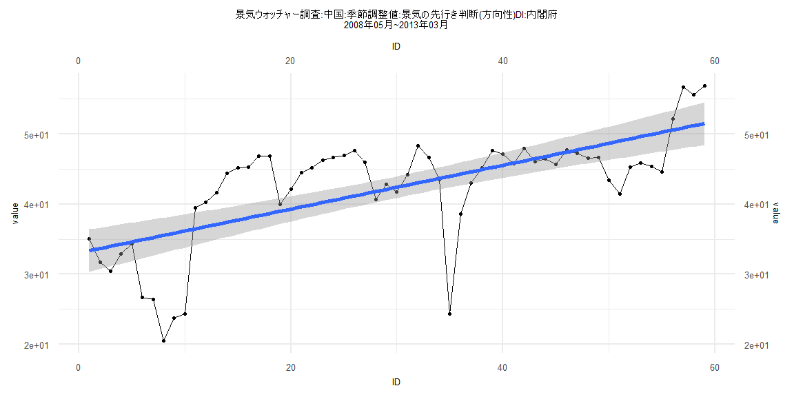
Call:
lm(formula = value ~ ID)

Residuals:
     Min       1Q   Median       3Q      Max
-19.7019  -1.8291   0.3559   4.5420   8.5308

Coefficients:
            Estimate Std. Error t value             Pr(>|t|)
(Intercept) 33.04944    1.56037  21.180 < 0.0000000000000002 ***
ID           0.31293    0.04523   6.918        0.00000000436 ***
---
Signif. codes:  0 '***' 0.001 '**' 0.01 '*' 0.05 '.' 0.1 ' ' 1

Residual standard error: 5.917 on 57 degrees of freedom
Multiple R-squared:  0.4564,    Adjusted R-squared:  0.4469
F-statistic: 47.86 on 1 and 57 DF,  p-value: 0.000000004355


    Two-sample Kolmogorov-Smirnov test

data:  lm_residuals and rnorm(n = length(lm_residuals), mean = 0, sd = sd(lm_residuals))
D = 0.23729, p-value = 0.07193
alternative hypothesis: two-sided


    Durbin-Watson test

data:  value ~ ID
DW = 0.61441, p-value = 0.00000000007821
alternative hypothesis: true autocorrelation is greater than 0


    studentized Breusch-Pagan test

data:  value ~ ID
BP = 2.4559, df = 1, p-value = 0.1171


    Box-Ljung test

data:  lm_residuals
X-squared = 29.096, df = 1, p-value = 0.00000006886
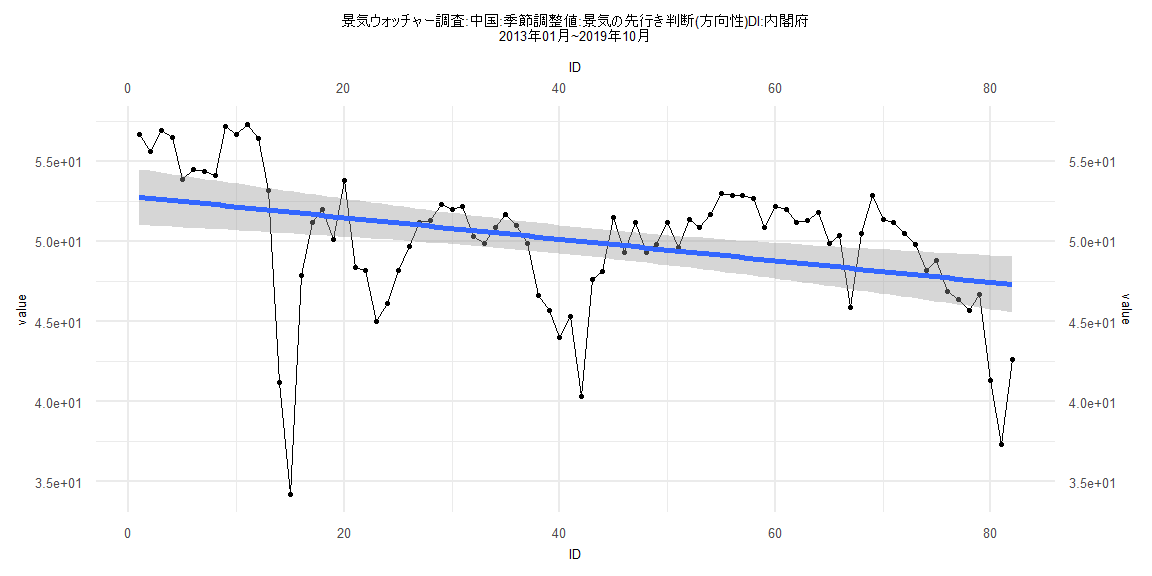
Call:
lm(formula = value ~ ID)

Residuals:
     Min       1Q   Median       3Q      Max
-17.1679  -1.5598   0.8128   2.4997   5.7072

Coefficients:
            Estimate Std. Error t value             Pr(>|t|)
(Intercept) 52.04255    0.90982  57.201 < 0.0000000000000002 ***
ID          -0.05622    0.01976  -2.845              0.00568 **
---
Signif. codes:  0 '***' 0.001 '**' 0.01 '*' 0.05 '.' 0.1 ' ' 1

Residual standard error: 4.005 on 77 degrees of freedom
Multiple R-squared:  0.09513,   Adjusted R-squared:  0.08338
F-statistic: 8.095 on 1 and 77 DF,  p-value: 0.005683


    Two-sample Kolmogorov-Smirnov test

data:  lm_residuals and rnorm(n = length(lm_residuals), mean = 0, sd = sd(lm_residuals))
D = 0.13924, p-value = 0.4302
alternative hypothesis: two-sided


    Durbin-Watson test

data:  value ~ ID
DW = 0.61962, p-value = 0.0000000000001376
alternative hypothesis: true autocorrelation is greater than 0


    studentized Breusch-Pagan test

data:  value ~ ID
BP = 1.3412, df = 1, p-value = 0.2468


    Box-Ljung test

data:  lm_residuals
X-squared = 37.027, df = 1, p-value = 0.000000001165