Analysis
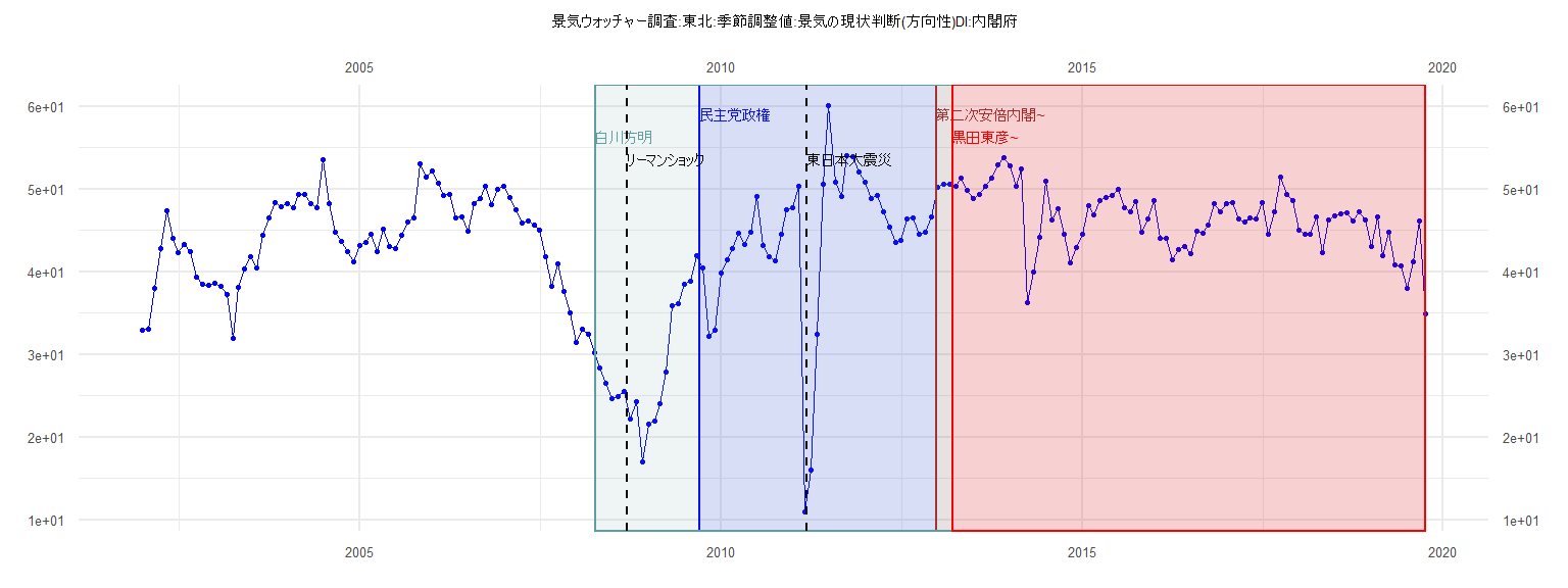
[1] "景気ウォッチャー調査:東北:季節調整値:景気の現状判断(方向性)DI:内閣府"
Jan Feb Mar Apr May Jun Jul Aug Sep Oct Nov Dec
2002 32.9 33.1 38.0 42.8 47.4 44.0 42.3 43.3 42.4 39.4 38.5 38.4
2003 38.6 38.3 37.2 32.0 38.1 40.3 41.8 40.5 44.4 46.5 48.4 47.9
2004 48.3 47.7 49.4 49.3 48.2 47.7 53.5 48.3 44.8 43.7 42.4 41.2
2005 43.2 43.6 44.5 42.5 45.2 43.1 42.8 44.4 46.0 46.5 53.1 51.5
2006 52.2 50.7 49.2 49.3 46.5 46.7 44.9 48.3 48.9 50.4 48.1 50.0
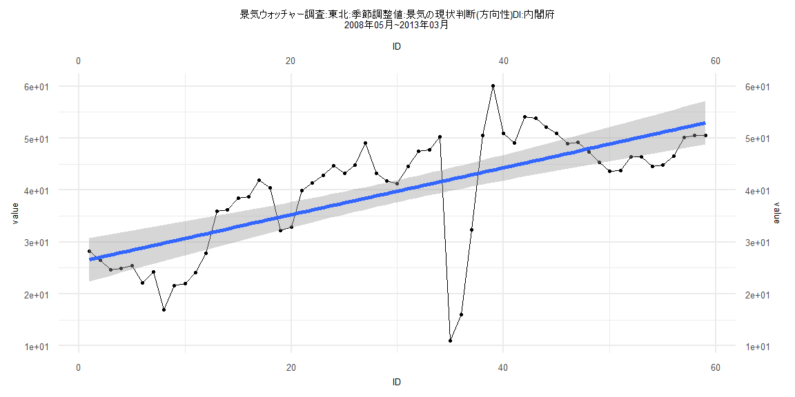
2007 50.4 49.0 47.5 45.9 46.1 45.7 45.0 41.8 38.2 40.9 37.6 35.0
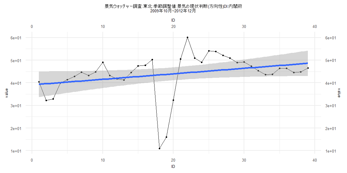
2008 31.5 33.1 32.4 30.2 28.3 26.5 24.7 24.9 25.5 22.2 24.3 17.0
2009 21.6 22.0 24.1 27.9 35.9 36.2 38.5 38.8 41.9 40.5 32.2 32.9
2010 39.9 41.4 42.8 44.7 43.3 44.8 49.1 43.2 41.8 41.3 44.6 47.5
2011 47.8 50.3 11.0 16.0 32.4 50.6 60.1 50.9 49.1 54.1 53.9 52.1
2012 50.9 48.9 49.2 47.3 45.4 43.6 43.8 46.4 46.5 44.6 44.8 46.6
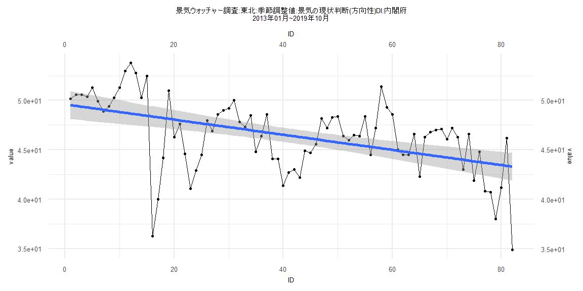
2013 50.2 50.6 50.6 50.4 51.3 49.9 48.9 49.4 50.3 51.3 53.0 53.8
2014 52.8 50.3 52.5 36.3 40.0 44.2 51.0 46.3 47.6 44.6 41.1 42.9
2015 44.5 48.0 46.9 48.6 49.0 49.2 50.0 47.8 47.3 48.5 44.8 46.4
2016 48.6 44.1 44.1 41.4 42.7 43.0 42.2 44.9 44.7 45.6 48.2 47.2
2017 48.3 48.4 46.4 46.0 46.5 46.4 48.4 44.5 47.2 51.4 49.3 48.6
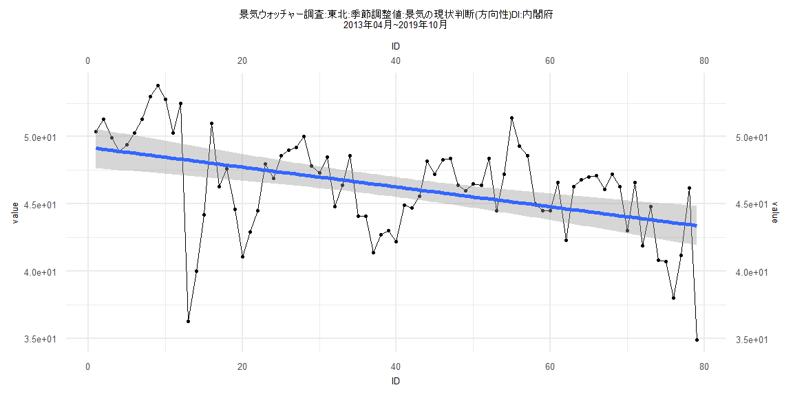
2018 45.0 44.5 44.5 46.6 42.3 46.3 46.8 47.0 47.1 46.1 47.2 46.3
2019 43.0 46.6 41.9 44.8 40.8 40.7 38.0 41.2 46.2 34.9
Call:
lm(formula = value ~ ID)

Residuals:
    Min      1Q  Median      3Q     Max
-32.520  -1.785   1.386   4.739  15.605

Coefficients:
            Estimate Std. Error t value             Pr(>|t|)
(Intercept)  39.1336     2.8880  13.551 0.000000000000000641 ***
ID            0.2437     0.1258   1.937               0.0605 .
---
Signif. codes:  0 '***' 0.001 '**' 0.01 '*' 0.05 '.' 0.1 ' ' 1

Residual standard error: 8.845 on 37 degrees of freedom
Multiple R-squared:  0.09203,   Adjusted R-squared:  0.06749
F-statistic:  3.75 on 1 and 37 DF,  p-value: 0.06046


    Two-sample Kolmogorov-Smirnov test

data:  lm_residuals and rnorm(n = length(lm_residuals), mean = 0, sd = sd(lm_residuals))
D = 0.25641, p-value = 0.1547
alternative hypothesis: two-sided


    Durbin-Watson test

data:  value ~ ID
DW = 0.904, p-value = 0.00003881
alternative hypothesis: true autocorrelation is greater than 0


    studentized Breusch-Pagan test

data:  value ~ ID
BP = 0.045699, df = 1, p-value = 0.8307


    Box-Ljung test

data:  lm_residuals
X-squared = 12.593, df = 1, p-value = 0.0003871
Call:
lm(formula = value ~ ID)

Residuals:
     Min       1Q   Median       3Q      Max
-12.0727  -1.9024   0.7359   2.1745   6.2484

Coefficients:
            Estimate Std. Error t value             Pr(>|t|)
(Intercept) 49.59982    0.72385  68.522 < 0.0000000000000002 ***
ID          -0.07669    0.01515  -5.062            0.0000026 ***
---
Signif. codes:  0 '***' 0.001 '**' 0.01 '*' 0.05 '.' 0.1 ' ' 1

Residual standard error: 3.247 on 80 degrees of freedom
Multiple R-squared:  0.2426,    Adjusted R-squared:  0.2331
F-statistic: 25.62 on 1 and 80 DF,  p-value: 0.000002598


    Two-sample Kolmogorov-Smirnov test

data:  lm_residuals and rnorm(n = length(lm_residuals), mean = 0, sd = sd(lm_residuals))
D = 0.14634, p-value = 0.3453
alternative hypothesis: two-sided


    Durbin-Watson test

data:  value ~ ID
DW = 1.0099, p-value = 0.000000394
alternative hypothesis: true autocorrelation is greater than 0


    studentized Breusch-Pagan test

data:  value ~ ID
BP = 0.33129, df = 1, p-value = 0.5649


    Box-Ljung test

data:  lm_residuals
X-squared = 17.441, df = 1, p-value = 0.00002964
Call:
lm(formula = value ~ ID)

Residuals:
    Min      1Q  Median      3Q     Max
-31.067  -3.732   1.671   5.860  16.217

Coefficients:
            Estimate Std. Error t value             Pr(>|t|)
(Intercept)  26.1751     2.1525  12.160 < 0.0000000000000002 ***
ID            0.4541     0.0624   7.277         0.0000000011 ***
---
Signif. codes:  0 '***' 0.001 '**' 0.01 '*' 0.05 '.' 0.1 ' ' 1

Residual standard error: 8.162 on 57 degrees of freedom
Multiple R-squared:  0.4816,    Adjusted R-squared:  0.4725
F-statistic: 52.95 on 1 and 57 DF,  p-value: 0.000000001101


    Two-sample Kolmogorov-Smirnov test

data:  lm_residuals and rnorm(n = length(lm_residuals), mean = 0, sd = sd(lm_residuals))
D = 0.13559, p-value = 0.6544
alternative hypothesis: two-sided


    Durbin-Watson test

data:  value ~ ID
DW = 0.74232, p-value = 0.000000009119
alternative hypothesis: true autocorrelation is greater than 0


    studentized Breusch-Pagan test

data:  value ~ ID
BP = 0.10718, df = 1, p-value = 0.7434


    Box-Ljung test

data:  lm_residuals
X-squared = 24.452, df = 1, p-value = 0.000000762
Call:
lm(formula = value ~ ID)

Residuals:
     Min       1Q   Median       3Q      Max
-11.9519  -2.0295   0.7265   2.2346   6.2415

Coefficients:
            Estimate Std. Error t value             Pr(>|t|)
(Intercept) 49.20935    0.75026   65.59 < 0.0000000000000002 ***
ID          -0.07365    0.01629   -4.52             0.000022 ***
---
Signif. codes:  0 '***' 0.001 '**' 0.01 '*' 0.05 '.' 0.1 ' ' 1

Residual standard error: 3.303 on 77 degrees of freedom
Multiple R-squared:  0.2097,    Adjusted R-squared:  0.1994
F-statistic: 20.43 on 1 and 77 DF,  p-value: 0.00002203


    Two-sample Kolmogorov-Smirnov test

data:  lm_residuals and rnorm(n = length(lm_residuals), mean = 0, sd = sd(lm_residuals))
D = 0.075949, p-value = 0.978
alternative hypothesis: two-sided


    Durbin-Watson test

data:  value ~ ID
DW = 1.0142, p-value = 0.0000006875
alternative hypothesis: true autocorrelation is greater than 0


    studentized Breusch-Pagan test

data:  value ~ ID
BP = 0.78093, df = 1, p-value = 0.3769


    Box-Ljung test

data:  lm_residuals
X-squared = 16.541, df = 1, p-value = 0.00004761