Analysis
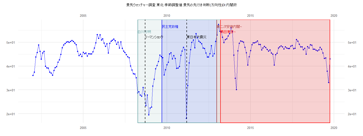
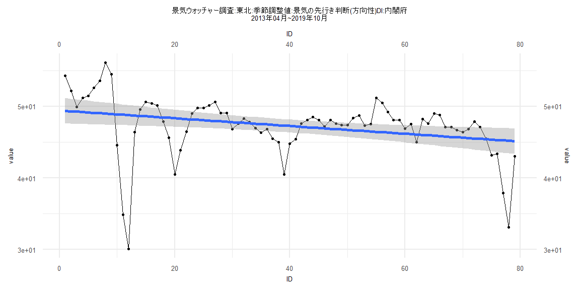
[1] "景気ウォッチャー調査:東北:季節調整値:景気の先行き判断(方向性)DI:内閣府"
      Jan  Feb  Mar  Apr  May  Jun  Jul  Aug  Sep  Oct  Nov  Dec
2002 36.1 37.5 43.8 45.7 48.9 46.2 42.9 45.5 46.2 40.0 39.3 39.2
2003 37.5 37.1 36.2 38.2 39.4 39.8 41.6 42.6 44.9 47.7 48.9 49.5
2004 50.1 50.3 50.0 50.4 50.8 50.4 49.7 49.0 46.2 44.4 45.0 44.0
2005 45.8 45.2 45.5 44.2 45.2 45.1 45.1 46.0 47.6 49.8 53.2 51.7
2006 53.1 51.0 51.5 49.7 48.3 49.4 45.5 49.6 50.5 50.9 51.4 50.7
2007 49.2 50.1 47.6 50.2 47.5 46.3 45.7 44.8 43.9 43.5 40.1 38.4
2008 36.8 36.7 35.1 28.8 29.3 27.9 27.4 31.0 28.4 23.4 27.9 19.5
2009 22.4 22.8 31.6 34.5 38.9 40.3 41.9 44.6 44.0 43.5 36.3 38.5
2010 40.6 41.6 45.1 45.6 43.0 44.4 43.2 39.1 39.2 39.9 44.5 46.3
2011 47.9 46.9 18.1 31.8 41.3 46.9 50.0 51.0 47.7 53.6 52.0 50.5
2012 50.0 49.4 47.6 47.4 45.5 43.8 43.8 45.2 48.6 44.2 45.2 50.4
2013 53.0 57.5 54.6 54.3 52.2 49.9 51.2 51.5 52.6 53.6 56.1 54.5
2014 44.6 34.9 30.1 46.4 49.6 50.6 50.4 50.1 47.9 45.6 40.5 43.9
2015 46.5 49.0 49.8 49.8 50.1 50.6 49.1 49.1 46.8 47.6 48.3 47.8
2016 47.0 46.3 46.8 45.5 45.0 40.5 44.8 45.4 47.6 48.1 48.5 48.1
2017 47.2 48.1 47.6 47.4 47.4 48.4 48.7 47.3 47.5 51.2 50.5 49.2
2018 48.1 48.1 46.9 47.5 45.0 48.2 47.6 49.0 48.8 47.1 47.1 46.7
2019 46.4 46.8 47.9 47.1 45.5 43.2 43.4 37.9 33.1 43.0
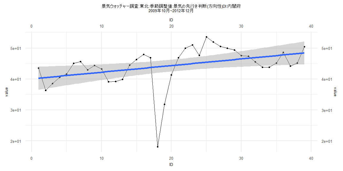
Call:
lm(formula = value ~ ID)

Residuals:
    Min      1Q  Median      3Q     Max
-25.819  -2.980   1.104   3.213   8.178

Coefficients:
            Estimate Std. Error t value            Pr(>|t|)
(Intercept) 40.05398    1.90743  20.999 <0.0000000000000002 ***
ID           0.21474    0.08312   2.584              0.0139 *
---
Signif. codes:  0 '***' 0.001 '**' 0.01 '*' 0.05 '.' 0.1 ' ' 1

Residual standard error: 5.842 on 37 degrees of freedom
Multiple R-squared:  0.1528,    Adjusted R-squared:  0.1299
F-statistic: 6.675 on 1 and 37 DF,  p-value: 0.01386


    Two-sample Kolmogorov-Smirnov test

data:  lm_residuals and rnorm(n = length(lm_residuals), mean = 0, sd = sd(lm_residuals))
D = 0.23077, p-value = 0.2523
alternative hypothesis: two-sided


    Durbin-Watson test

data:  value ~ ID
DW = 1.1087, p-value = 0.0008298
alternative hypothesis: true autocorrelation is greater than 0


    studentized Breusch-Pagan test

data:  value ~ ID
BP = 0.015726, df = 1, p-value = 0.9002


    Box-Ljung test

data:  lm_residuals
X-squared = 8.1447, df = 1, p-value = 0.004319
Call:
lm(formula = value ~ ID)

Residuals:
     Min       1Q   Median       3Q      Max
-19.2591  -1.0196   0.9533   1.8696   7.2504

Coefficients:
            Estimate Std. Error t value             Pr(>|t|)
(Intercept) 50.38663    0.91039  55.346 < 0.0000000000000002 ***
ID          -0.06850    0.01906  -3.595              0.00056 ***
---
Signif. codes:  0 '***' 0.001 '**' 0.01 '*' 0.05 '.' 0.1 ' ' 1

Residual standard error: 4.084 on 80 degrees of freedom
Multiple R-squared:  0.1391,    Adjusted R-squared:  0.1283
F-statistic: 12.92 on 1 and 80 DF,  p-value: 0.0005598


    Two-sample Kolmogorov-Smirnov test

data:  lm_residuals and rnorm(n = length(lm_residuals), mean = 0, sd = sd(lm_residuals))
D = 0.31707, p-value = 0.0004799
alternative hypothesis: two-sided


    Durbin-Watson test

data:  value ~ ID
DW = 0.65039, p-value = 0.0000000000002787
alternative hypothesis: true autocorrelation is greater than 0


    studentized Breusch-Pagan test

data:  value ~ ID
BP = 2.1074, df = 1, p-value = 0.1466


    Box-Ljung test

data:  lm_residuals
X-squared = 38.28, df = 1, p-value = 0.0000000006129
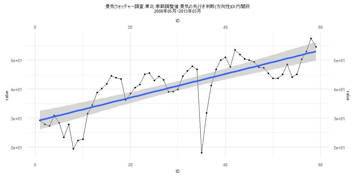
Call:
lm(formula = value ~ ID)

Residuals:
     Min       1Q   Median       3Q      Max
-25.1389  -2.6657   0.7674   4.4711   9.1283

Coefficients:
            Estimate Std. Error t value             Pr(>|t|)
(Intercept) 28.93086    1.63792   17.66 < 0.0000000000000002 ***
ID           0.40880    0.04748    8.61     0.00000000000674 ***
---
Signif. codes:  0 '***' 0.001 '**' 0.01 '*' 0.05 '.' 0.1 ' ' 1

Residual standard error: 6.211 on 57 degrees of freedom
Multiple R-squared:  0.5653,    Adjusted R-squared:  0.5577
F-statistic: 74.13 on 1 and 57 DF,  p-value: 0.000000000006737


    Two-sample Kolmogorov-Smirnov test

data:  lm_residuals and rnorm(n = length(lm_residuals), mean = 0, sd = sd(lm_residuals))
D = 0.13559, p-value = 0.6544
alternative hypothesis: two-sided


    Durbin-Watson test

data:  value ~ ID
DW = 0.76844, p-value = 0.00000002117
alternative hypothesis: true autocorrelation is greater than 0


    studentized Breusch-Pagan test

data:  value ~ ID
BP = 0.13189, df = 1, p-value = 0.7165


    Box-Ljung test

data:  lm_residuals
X-squared = 23.487, df = 1, p-value = 0.000001257
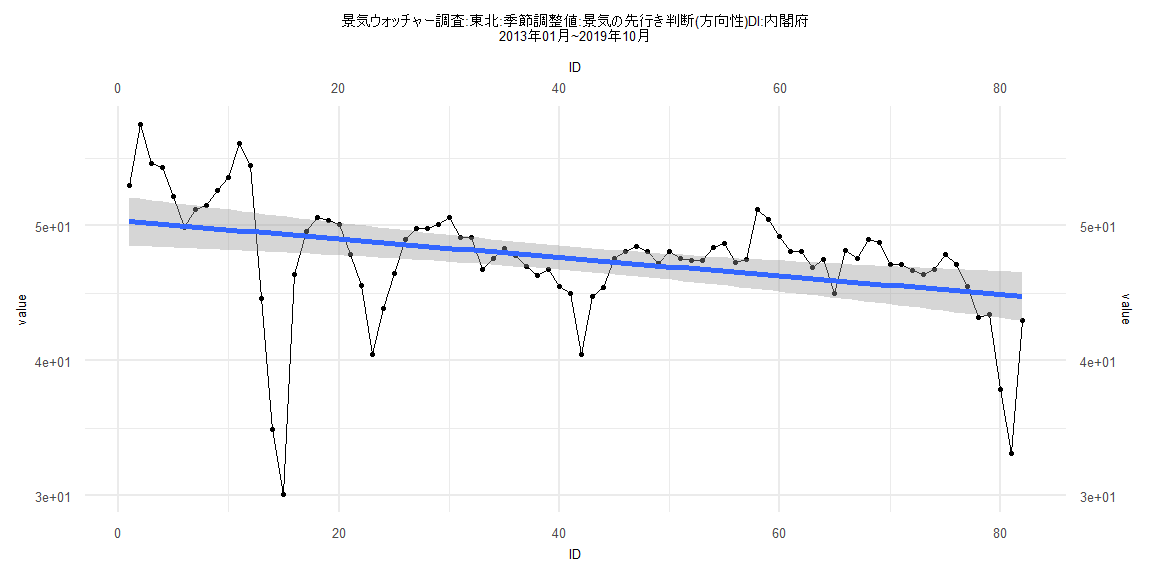
Call:
lm(formula = value ~ ID)

Residuals:
     Min       1Q   Median       3Q      Max
-18.6776  -1.0342   0.9996   1.8550   7.1055

Coefficients:
            Estimate Std. Error t value             Pr(>|t|)
(Intercept) 49.42824    0.91320  54.127 < 0.0000000000000002 ***
ID          -0.05422    0.01983  -2.734              0.00777 **
---
Signif. codes:  0 '***' 0.001 '**' 0.01 '*' 0.05 '.' 0.1 ' ' 1

Residual standard error: 4.02 on 77 degrees of freedom
Multiple R-squared:  0.08847,   Adjusted R-squared:  0.07663
F-statistic: 7.473 on 1 and 77 DF,  p-value: 0.007766


    Two-sample Kolmogorov-Smirnov test

data:  lm_residuals and rnorm(n = length(lm_residuals), mean = 0, sd = sd(lm_residuals))
D = 0.18987, p-value = 0.116
alternative hypothesis: two-sided


    Durbin-Watson test

data:  value ~ ID
DW = 0.67446, p-value = 0.000000000002355
alternative hypothesis: true autocorrelation is greater than 0


    studentized Breusch-Pagan test

data:  value ~ ID
BP = 2.0083, df = 1, p-value = 0.1564


    Box-Ljung test

data:  lm_residuals
X-squared = 34.786, df = 1, p-value = 0.00000000368