Analysis
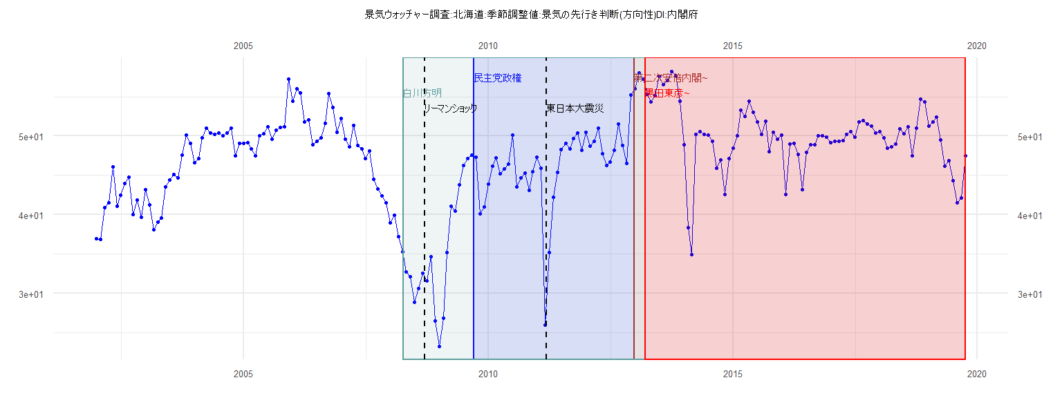
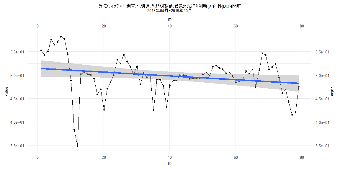
[1] "景気ウォッチャー調査:北海道:季節調整値:景気の先行き判断(方向性)DI:内閣府"
      Jan  Feb  Mar  Apr  May  Jun  Jul  Aug  Sep  Oct  Nov  Dec
2002 37.0 36.9 40.9 41.5 46.1 41.1 42.5 44.0 44.8 40.0 41.9 39.7
2003 43.2 41.3 38.1 39.1 39.6 43.5 44.4 45.1 44.7 47.6 50.1 49.1
2004 46.6 47.1 49.8 51.0 50.4 50.2 50.4 50.0 50.4 51.0 47.5 49.1
2005 49.1 49.2 48.4 47.5 50.0 50.3 51.2 49.6 50.7 51.1 51.2 57.2
2006 54.4 56.0 55.5 51.8 52.1 48.9 49.3 49.8 51.6 55.4 53.6 50.5
2007 52.2 49.6 48.6 51.4 48.8 48.4 47.1 48.1 44.5 43.3 42.4 41.5
2008 39.0 39.9 37.2 35.3 32.7 32.1 28.9 30.6 32.6 31.6 34.7 26.5
2009 23.3 26.9 35.2 41.1 40.5 43.8 46.3 47.1 47.6 47.3 40.1 41.0
2010 43.9 46.2 47.2 45.2 45.8 46.4 50.1 43.5 44.7 45.3 43.1 45.5
2011 47.3 45.9 26.0 35.2 42.2 45.4 48.3 49.1 48.4 49.7 50.4 48.2
2012 50.5 48.7 49.3 51.0 47.8 46.3 46.7 48.2 51.5 48.8 46.5 55.2
2013 56.0 58.0 57.2 55.3 54.3 55.1 57.6 56.5 57.1 58.2 57.7 54.4
2014 48.9 38.4 34.9 50.2 50.6 50.2 50.1 49.3 45.9 47.0 42.6 47.1
2015 48.5 50.0 53.3 52.5 54.4 53.0 51.8 50.2 51.9 48.0 50.5 49.6
2016 50.1 42.6 49.0 49.1 47.7 43.2 47.9 48.9 48.9 50.0 50.0 49.9
2017 49.2 49.3 49.3 49.4 50.2 50.6 49.9 51.8 52.0 51.5 51.3 50.4
2018 50.6 49.8 48.5 48.6 49.0 50.9 50.3 51.2 47.5 51.0 54.7 54.3
2019 51.3 51.8 52.4 49.5 46.2 46.9 44.3 41.5 42.1 47.5
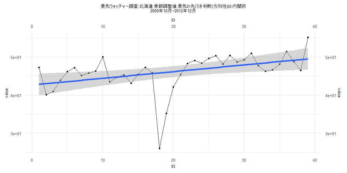
Call:
lm(formula = value ~ ID)

Residuals:
     Min       1Q   Median       3Q      Max
-19.8501  -1.0477   0.7639   2.4234   5.6596

Coefficients:
            Estimate Std. Error t value             Pr(>|t|)
(Intercept) 42.67827    1.45419  29.349 < 0.0000000000000002 ***
ID           0.17621    0.06337   2.781              0.00848 **
---
Signif. codes:  0 '***' 0.001 '**' 0.01 '*' 0.05 '.' 0.1 ' ' 1

Residual standard error: 4.454 on 37 degrees of freedom
Multiple R-squared:  0.1729,    Adjusted R-squared:  0.1505
F-statistic: 7.734 on 1 and 37 DF,  p-value: 0.008476


    Two-sample Kolmogorov-Smirnov test

data:  lm_residuals and rnorm(n = length(lm_residuals), mean = 0, sd = sd(lm_residuals))
D = 0.25641, p-value = 0.1547
alternative hypothesis: two-sided


    Durbin-Watson test

data:  value ~ ID
DW = 1.1277, p-value = 0.001054
alternative hypothesis: true autocorrelation is greater than 0


    studentized Breusch-Pagan test

data:  value ~ ID
BP = 0.047597, df = 1, p-value = 0.8273


    Box-Ljung test

data:  lm_residuals
X-squared = 6.7646, df = 1, p-value = 0.009299
Call:
lm(formula = value ~ ID)

Residuals:
     Min       1Q   Median       3Q      Max
-16.6578  -1.2281   0.1496   2.4474   6.3675

Coefficients:
            Estimate Std. Error t value             Pr(>|t|)
(Intercept) 52.38166    0.89400  58.593 < 0.0000000000000002 ***
ID          -0.05492    0.01871  -2.935              0.00435 **
---
Signif. codes:  0 '***' 0.001 '**' 0.01 '*' 0.05 '.' 0.1 ' ' 1

Residual standard error: 4.011 on 80 degrees of freedom
Multiple R-squared:  0.09721,   Adjusted R-squared:  0.08593
F-statistic: 8.614 on 1 and 80 DF,  p-value: 0.004352


    Two-sample Kolmogorov-Smirnov test

data:  lm_residuals and rnorm(n = length(lm_residuals), mean = 0, sd = sd(lm_residuals))
D = 0.15854, p-value = 0.2552
alternative hypothesis: two-sided


    Durbin-Watson test

data:  value ~ ID
DW = 0.61481, p-value = 0.00000000000003916
alternative hypothesis: true autocorrelation is greater than 0


    studentized Breusch-Pagan test

data:  value ~ ID
BP = 4.2694, df = 1, p-value = 0.0388


    Box-Ljung test

data:  lm_residuals
X-squared = 40.17, df = 1, p-value = 0.0000000002328
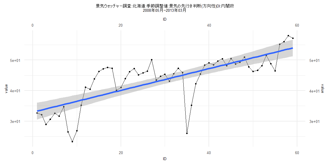
Call:
lm(formula = value ~ ID)

Residuals:
    Min      1Q  Median      3Q     Max
-19.421  -2.367   0.839   3.072   8.600

Coefficients:
            Estimate Std. Error t value             Pr(>|t|)
(Intercept) 32.93618    1.39993   23.53 < 0.0000000000000002 ***
ID           0.35670    0.04058    8.79     0.00000000000341 ***
---
Signif. codes:  0 '***' 0.001 '**' 0.01 '*' 0.05 '.' 0.1 ' ' 1

Residual standard error: 5.308 on 57 degrees of freedom
Multiple R-squared:  0.5754,    Adjusted R-squared:  0.568
F-statistic: 77.26 on 1 and 57 DF,  p-value: 0.000000000003411


    Two-sample Kolmogorov-Smirnov test

data:  lm_residuals and rnorm(n = length(lm_residuals), mean = 0, sd = sd(lm_residuals))
D = 0.13559, p-value = 0.6544
alternative hypothesis: two-sided


    Durbin-Watson test

data:  value ~ ID
DW = 0.66314, p-value = 0.0000000005495
alternative hypothesis: true autocorrelation is greater than 0


    studentized Breusch-Pagan test

data:  value ~ ID
BP = 1.1975, df = 1, p-value = 0.2738


    Box-Ljung test

data:  lm_residuals
X-squared = 27.449, df = 1, p-value = 0.0000001613
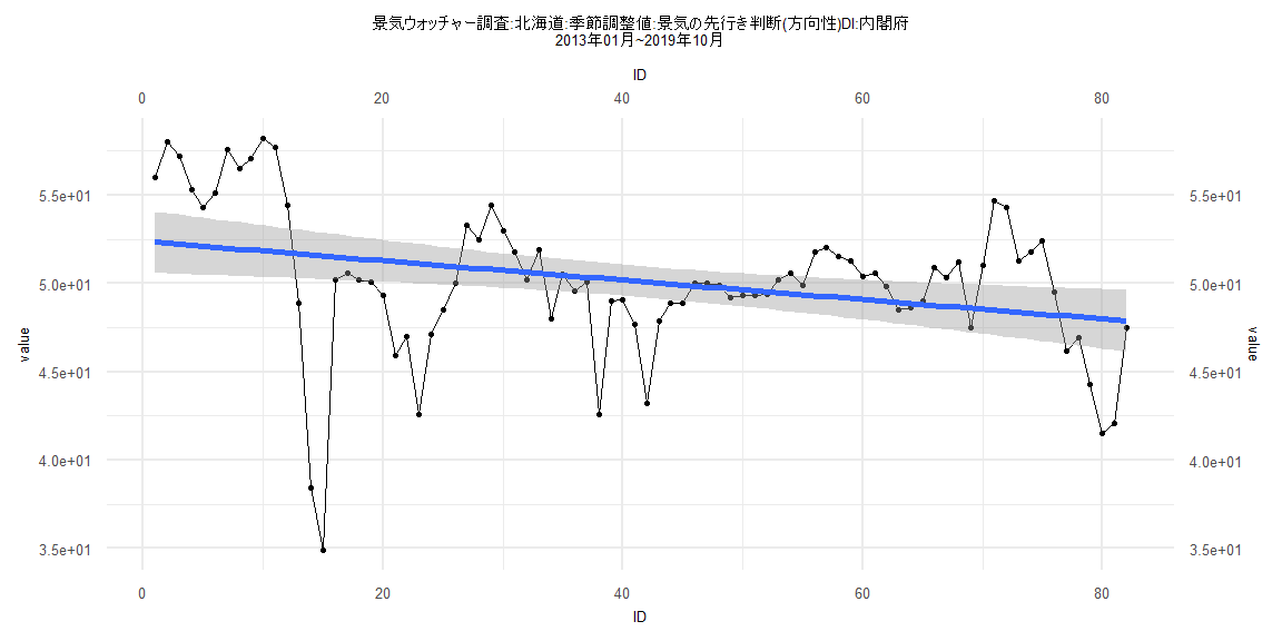
Call:
lm(formula = value ~ ID)

Residuals:
     Min       1Q   Median       3Q      Max
-16.0747  -1.1414   0.0551   2.3240   7.0223

Coefficients:
            Estimate Std. Error t value            Pr(>|t|)
(Intercept) 51.46183    0.89857   57.27 <0.0000000000000002 ***
ID          -0.04060    0.01952   -2.08              0.0408 *
---
Signif. codes:  0 '***' 0.001 '**' 0.01 '*' 0.05 '.' 0.1 ' ' 1

Residual standard error: 3.955 on 77 degrees of freedom
Multiple R-squared:  0.05321,   Adjusted R-squared:  0.04091
F-statistic: 4.327 on 1 and 77 DF,  p-value: 0.04083


    Two-sample Kolmogorov-Smirnov test

data:  lm_residuals and rnorm(n = length(lm_residuals), mean = 0, sd = sd(lm_residuals))
D = 0.16456, p-value = 0.2361
alternative hypothesis: two-sided


    Durbin-Watson test

data:  value ~ ID
DW = 0.65005, p-value = 0.0000000000006906
alternative hypothesis: true autocorrelation is greater than 0


    studentized Breusch-Pagan test

data:  value ~ ID
BP = 4.8308, df = 1, p-value = 0.02796


    Box-Ljung test

data:  lm_residuals
X-squared = 36.662, df = 1, p-value = 0.000000001405