Analysis
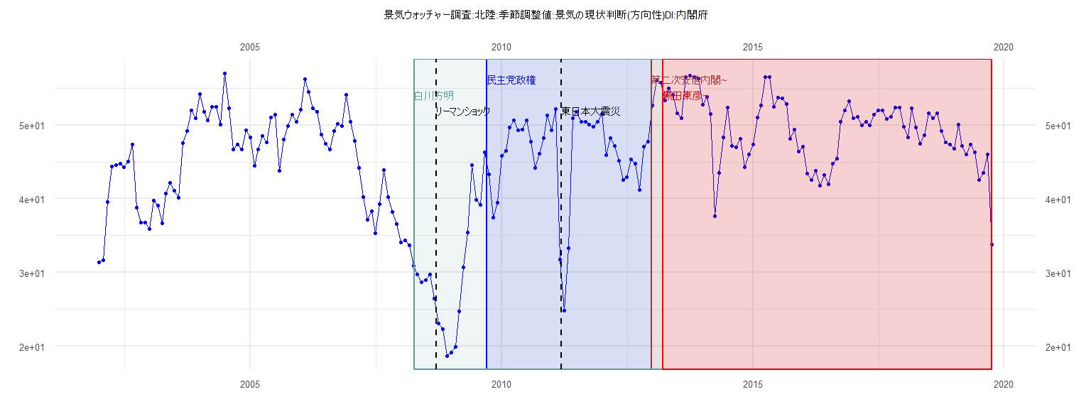
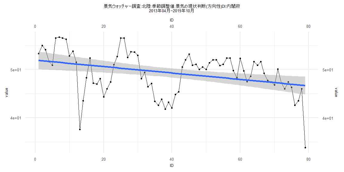
[1] "景気ウォッチャー調査:北陸:季節調整値:景気の現状判断(方向性)DI:内閣府"
      Jan  Feb  Mar  Apr  May  Jun  Jul  Aug  Sep  Oct  Nov  Dec
2002 31.4 31.7 39.6 44.4 44.6 44.8 44.3 45.1 47.4 38.8 36.8 36.8
2003 35.9 39.8 39.1 36.7 40.7 42.2 41.1 40.1 47.6 49.2 52.0 50.9
2004 54.2 51.8 50.6 52.5 52.5 50.1 57.0 52.3 46.7 47.4 46.7 49.3
2005 48.3 44.5 46.7 48.5 47.7 51.0 51.4 43.8 48.0 49.9 51.4 50.5
2006 52.1 56.2 54.5 52.3 51.8 48.7 47.5 46.7 49.2 50.2 49.9 54.1
2007 50.5 47.9 44.2 40.2 37.2 38.3 35.3 39.3 43.9 40.2 38.2 36.6
2008 34.1 34.4 33.7 30.9 29.7 28.7 29.0 29.7 26.5 23.1 22.3 18.7
2009 19.1 19.9 24.7 30.7 35.4 44.6 39.9 39.2 46.3 43.3 37.4 39.5
2010 45.8 46.5 49.7 50.6 49.3 49.4 50.6 47.8 44.2 46.1 48.2 51.3
2011 49.3 52.2 31.8 24.8 33.3 50.9 51.8 50.5 50.5 50.1 49.8 50.5
2012 51.5 45.9 48.2 47.2 45.2 42.6 42.9 45.3 44.8 41.2 47.1 47.8
2013 52.7 56.0 55.8 53.3 55.0 54.1 51.6 50.9 56.5 56.7 56.5 56.3
2014 52.8 53.8 51.5 37.6 43.5 48.3 52.4 47.2 47.0 48.1 44.3 46.0
2015 47.4 51.0 52.7 56.5 56.5 52.5 53.7 53.6 52.9 48.1 49.4 46.4
2016 47.1 43.4 42.6 43.8 41.8 43.2 42.0 44.8 45.4 50.5 52.0 53.2
2017 50.9 51.1 50.0 50.5 50.0 51.4 52.0 52.0 50.8 51.1 52.4 52.4
2018 49.8 48.3 52.3 49.7 47.5 48.6 51.6 50.9 51.6 49.2 47.7 47.4
2019 46.8 50.1 47.2 46.0 47.4 46.3 42.6 43.5 46.0 33.8
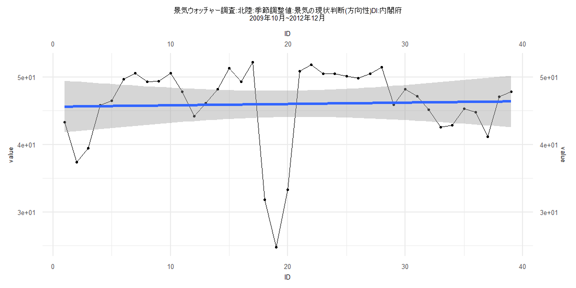
Call:
lm(formula = value ~ ID)

Residuals:
    Min      1Q  Median      3Q     Max
-21.203  -1.604   1.393   4.156   6.238

Coefficients:
            Estimate Std. Error t value            Pr(>|t|)
(Intercept) 45.61862    1.96405  23.227 <0.0000000000000002 ***
ID           0.02022    0.08558   0.236               0.815
---
Signif. codes:  0 '***' 0.001 '**' 0.01 '*' 0.05 '.' 0.1 ' ' 1

Residual standard error: 6.015 on 37 degrees of freedom
Multiple R-squared:  0.001507,  Adjusted R-squared:  -0.02548
F-statistic: 0.05584 on 1 and 37 DF,  p-value: 0.8145


    Two-sample Kolmogorov-Smirnov test

data:  lm_residuals and rnorm(n = length(lm_residuals), mean = 0, sd = sd(lm_residuals))
D = 0.20513, p-value = 0.3888
alternative hypothesis: two-sided


    Durbin-Watson test

data:  value ~ ID
DW = 0.8205, p-value = 0.000008207
alternative hypothesis: true autocorrelation is greater than 0


    studentized Breusch-Pagan test

data:  value ~ ID
BP = 0.22105, df = 1, p-value = 0.6382


    Box-Ljung test

data:  lm_residuals
X-squared = 14.498, df = 1, p-value = 0.0001403
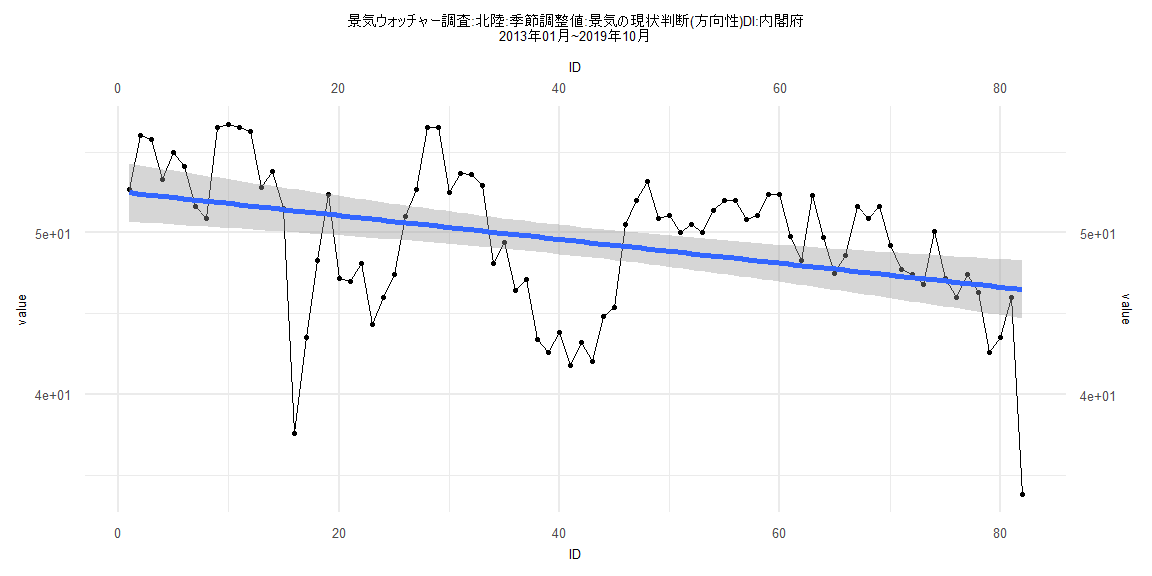
Call:
lm(formula = value ~ ID)

Residuals:
    Min      1Q  Median      3Q     Max
-13.761  -2.792   1.135   2.906   6.098

Coefficients:
            Estimate Std. Error t value             Pr(>|t|)
(Intercept) 52.54201    0.91958  57.137 < 0.0000000000000002 ***
ID          -0.07380    0.01925  -3.834              0.00025 ***
---
Signif. codes:  0 '***' 0.001 '**' 0.01 '*' 0.05 '.' 0.1 ' ' 1

Residual standard error: 4.126 on 80 degrees of freedom
Multiple R-squared:  0.1552,    Adjusted R-squared:  0.1447
F-statistic:  14.7 on 1 and 80 DF,  p-value: 0.0002499


    Two-sample Kolmogorov-Smirnov test

data:  lm_residuals and rnorm(n = length(lm_residuals), mean = 0, sd = sd(lm_residuals))
D = 0.15854, p-value = 0.2552
alternative hypothesis: two-sided


    Durbin-Watson test

data:  value ~ ID
DW = 0.58504, p-value = 0.000000000000006782
alternative hypothesis: true autocorrelation is greater than 0


    studentized Breusch-Pagan test

data:  value ~ ID
BP = 0.3062, df = 1, p-value = 0.58


    Box-Ljung test

data:  lm_residuals
X-squared = 35.743, df = 1, p-value = 0.000000002251
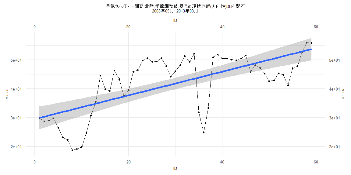
Call:
lm(formula = value ~ ID)

Residuals:
    Min      1Q  Median      3Q     Max
-19.476  -5.012   1.795   6.117  11.252

Coefficients:
            Estimate Std. Error t value             Pr(>|t|)
(Intercept) 29.49205    2.00150  14.735 < 0.0000000000000002 ***
ID           0.41066    0.05802   7.078        0.00000000236 ***
---
Signif. codes:  0 '***' 0.001 '**' 0.01 '*' 0.05 '.' 0.1 ' ' 1

Residual standard error: 7.589 on 57 degrees of freedom
Multiple R-squared:  0.4678,    Adjusted R-squared:  0.4584
F-statistic:  50.1 on 1 and 57 DF,  p-value: 0.00000000236


    Two-sample Kolmogorov-Smirnov test

data:  lm_residuals and rnorm(n = length(lm_residuals), mean = 0, sd = sd(lm_residuals))
D = 0.11864, p-value = 0.8052
alternative hypothesis: two-sided


    Durbin-Watson test

data:  value ~ ID
DW = 0.42869, p-value = 0.000000000000005205
alternative hypothesis: true autocorrelation is greater than 0


    studentized Breusch-Pagan test

data:  value ~ ID
BP = 1.867, df = 1, p-value = 0.1718


    Box-Ljung test

data:  lm_residuals
X-squared = 38.237, df = 1, p-value = 0.0000000006265
Call:
lm(formula = value ~ ID)

Residuals:
    Min      1Q  Median      3Q     Max
-13.473  -2.608   1.257   2.923   6.292

Coefficients:
            Estimate Std. Error t value             Pr(>|t|)
(Intercept) 51.93905    0.94542  54.937 < 0.0000000000000002 ***
ID          -0.06658    0.02053  -3.242              0.00175 **
---
Signif. codes:  0 '***' 0.001 '**' 0.01 '*' 0.05 '.' 0.1 ' ' 1

Residual standard error: 4.162 on 77 degrees of freedom
Multiple R-squared:  0.1201,    Adjusted R-squared:  0.1087
F-statistic: 10.51 on 1 and 77 DF,  p-value: 0.001753


    Two-sample Kolmogorov-Smirnov test

data:  lm_residuals and rnorm(n = length(lm_residuals), mean = 0, sd = sd(lm_residuals))
D = 0.1519, p-value = 0.3233
alternative hypothesis: two-sided


    Durbin-Watson test

data:  value ~ ID
DW = 0.58451, p-value = 0.00000000000001885
alternative hypothesis: true autocorrelation is greater than 0


    studentized Breusch-Pagan test

data:  value ~ ID
BP = 0.56371, df = 1, p-value = 0.4528


    Box-Ljung test

data:  lm_residuals
X-squared = 34.108, df = 1, p-value = 0.000000005214