Analysis
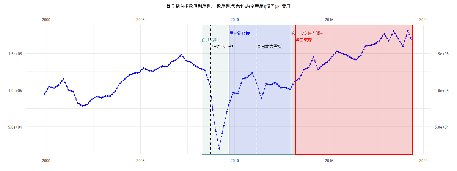
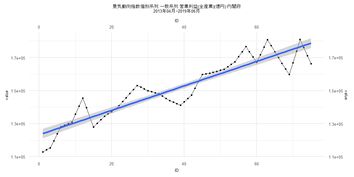
[1] "景気動向指数個別系列:一致系列:営業利益(全産業)(億円):内閣府"
        Jan    Feb    Mar    Apr    May    Jun    Jul    Aug    Sep    Oct    Nov    Dec
1999                                                                               94921
2000  98261 101601 104941 104275 103609 102943 104307 105672 107036 109835 112633 115432
2001 110445 105457 100470  99746  99021  98297  93112  87926  82741  81337  79933  78529
2002  79151  79772  80394  82833  85273  87712  88914  90116  91318  90743  90168  89593
2003  90333  91073  91813  91890  91968  92045  94364  96684  99003 102507 106010 109514
2004 111346 113179 115011 116921 118830 120740 121543 122345 123148 123412 123677 123941
2005 125982 128024 130065 128962 127858 126755 126494 126232 125971 127191 128411 129631
2006 130675 131720 132764 132646 132527 132409 134583 136756 138930 139903 140876 141849
2007 144056 146264 148471 145663 142856 140048 139424 138800 138176 136404 134632 132860
2008 131751 130641 129532 128685 127837 126990 120652 114314 107976  90498  73019  55541
2009  43727  31912  20098  30645  41193  51740  61155  70571  79986  85403  90819  96236
2010  95985  95734  95483 102250 109017 115784 116288 116793 117297 119412 121528 123643
2011 118873 114104 109334 102600  95865  89131  95667 102203 108739 108245 107750 107256
2012 108421 109587 110752 108273 105793 103314 103489 103664 103839 102958 102077 101196
2013 104674 108152 111630 112877 114124 115371 119615 123858 128102 129065 130027 130990
2014 135788 140585 145383 139593 133803 128013 130169 132325 134481 135879 137278 138676
2015 141023 143371 145718 148185 150653 153120 152083 151045 150008 149354 148700 148046
2016 146676 145307 143937 143035 142132 141230 143262 145294 147326 151490 155655 159819
2017 160217 160614 161012 161660 162307 162955 164434 165914 167393 170509 173624 176740
2018 173567 170394 167221 171755 176288 180822 177204 173587 169969 166551 163134 159716
2019 166812 173909 181005 176095 171184 166274
Call:
lm(formula = value ~ ID)

Residuals:
     Min       1Q   Median       3Q      Max
-19156.6  -5300.5   -731.9   4183.7  18195.8

Coefficients:
            Estimate Std. Error t value            Pr(>|t|)
(Intercept) 104496.2     3009.4  34.723 <0.0000000000000002 ***
ID              63.4      131.1   0.483               0.632
---
Signif. codes:  0 '***' 0.001 '**' 0.01 '*' 0.05 '.' 0.1 ' ' 1

Residual standard error: 9217 on 37 degrees of freedom
Multiple R-squared:  0.006278,  Adjusted R-squared:  -0.02058
F-statistic: 0.2337 on 1 and 37 DF,  p-value: 0.6316


    Two-sample Kolmogorov-Smirnov test

data:  lm_residuals and rnorm(n = length(lm_residuals), mean = 0, sd = sd(lm_residuals))
D = 0.23077, p-value = 0.2523
alternative hypothesis: two-sided


    Durbin-Watson test

data:  value ~ ID
DW = 0.18031, p-value < 0.00000000000000022
alternative hypothesis: true autocorrelation is greater than 0


    studentized Breusch-Pagan test

data:  value ~ ID
BP = 11.6, df = 1, p-value = 0.0006594


    Box-Ljung test

data:  lm_residuals
X-squared = 30.128, df = 1, p-value = 0.00000004044
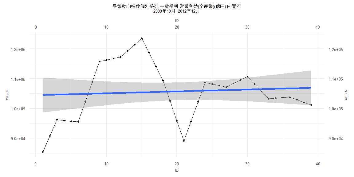
Call:
lm(formula = value ~ ID)

Residuals:
   Min     1Q Median     3Q    Max
-15438  -4866   1766   3955  14799

Coefficients:
             Estimate Std. Error t value            Pr(>|t|)
(Intercept) 118854.91    1564.71   75.96 <0.0000000000000002 ***
ID             781.92      34.41   22.72 <0.0000000000000002 ***
---
Signif. codes:  0 '***' 0.001 '**' 0.01 '*' 0.05 '.' 0.1 ' ' 1

Residual standard error: 6843 on 76 degrees of freedom
Multiple R-squared:  0.8717,    Adjusted R-squared:   0.87
F-statistic: 516.2 on 1 and 76 DF,  p-value: < 0.00000000000000022


    Two-sample Kolmogorov-Smirnov test

data:  lm_residuals and rnorm(n = length(lm_residuals), mean = 0, sd = sd(lm_residuals))
D = 0.12821, p-value = 0.546
alternative hypothesis: two-sided


    Durbin-Watson test

data:  value ~ ID
DW = 0.21484, p-value < 0.00000000000000022
alternative hypothesis: true autocorrelation is greater than 0


    studentized Breusch-Pagan test

data:  value ~ ID
BP = 0.11212, df = 1, p-value = 0.7377


    Box-Ljung test

data:  lm_residuals
X-squared = 56.537, df = 1, p-value = 0.00000000000005518
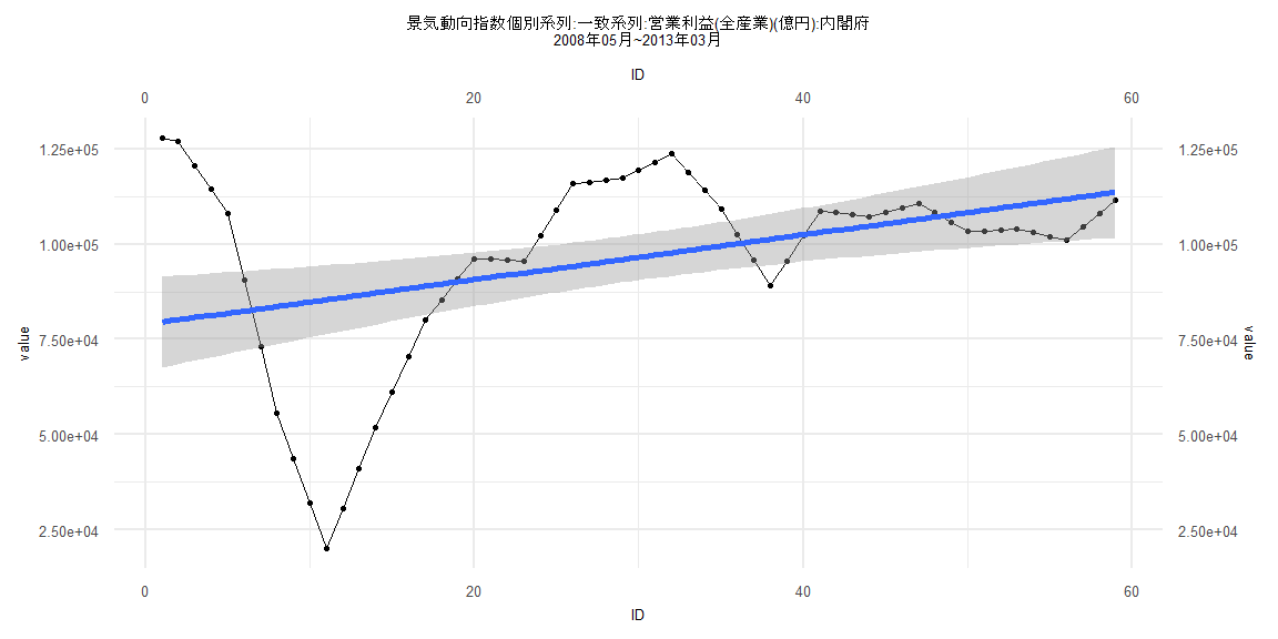
Call:
lm(formula = value ~ ID)

Residuals:
   Min     1Q Median     3Q    Max
-65303  -7723   2472  12515  48309

Coefficients:
            Estimate Std. Error t value            Pr(>|t|)
(Intercept)  78940.2     6113.9  12.912 <0.0000000000000002 ***
ID             587.4      177.2   3.314              0.0016 **
---
Signif. codes:  0 '***' 0.001 '**' 0.01 '*' 0.05 '.' 0.1 ' ' 1

Residual standard error: 23180 on 57 degrees of freedom
Multiple R-squared:  0.1616,    Adjusted R-squared:  0.1468
F-statistic: 10.98 on 1 and 57 DF,  p-value: 0.001602


    Two-sample Kolmogorov-Smirnov test

data:  lm_residuals and rnorm(n = length(lm_residuals), mean = 0, sd = sd(lm_residuals))
D = 0.13559, p-value = 0.6544
alternative hypothesis: two-sided


    Durbin-Watson test

data:  value ~ ID
DW = 0.089094, p-value < 0.00000000000000022
alternative hypothesis: true autocorrelation is greater than 0


    studentized Breusch-Pagan test

data:  value ~ ID
BP = 20.604, df = 1, p-value = 0.000005647


    Box-Ljung test

data:  lm_residuals
X-squared = 52.213, df = 1, p-value = 0.000000000000498
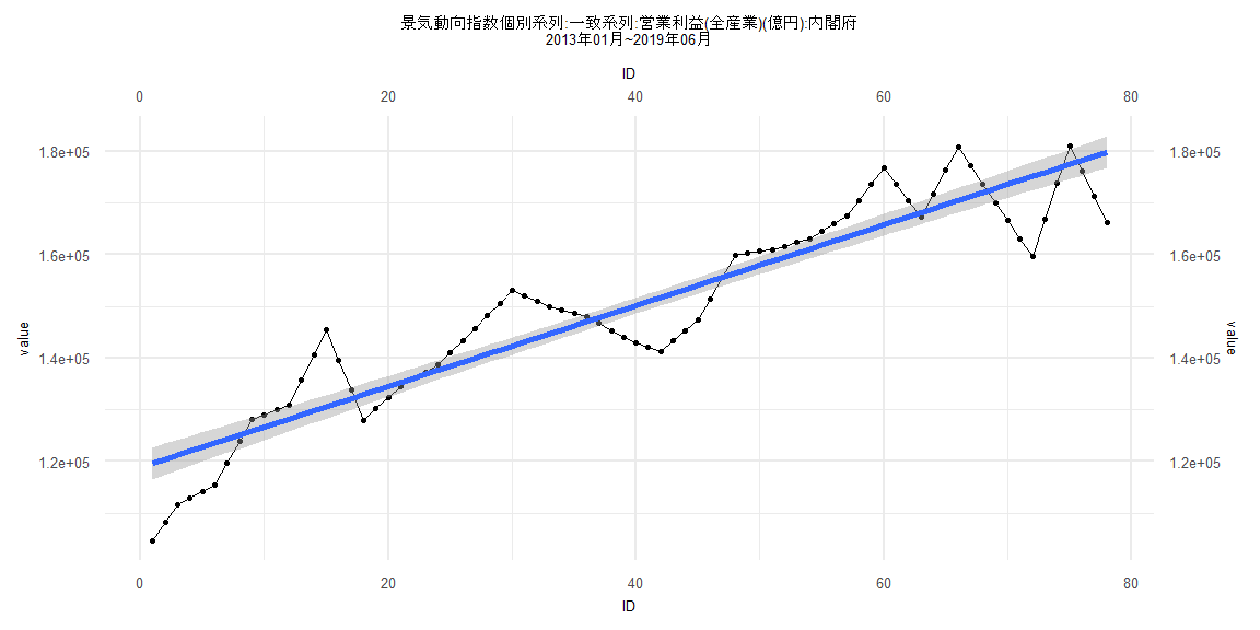
Call:
lm(formula = value ~ ID)

Residuals:
     Min       1Q   Median       3Q      Max
-14657.6  -4404.7    850.7   4271.0  13243.0

Coefficients:
             Estimate Std. Error t value            Pr(>|t|)
(Intercept) 123248.76    1499.39   82.20 <0.0000000000000002 ***
ID             740.94      34.28   21.61 <0.0000000000000002 ***
---
Signif. codes:  0 '***' 0.001 '**' 0.01 '*' 0.05 '.' 0.1 ' ' 1

Residual standard error: 6428 on 73 degrees of freedom
Multiple R-squared:  0.8648,    Adjusted R-squared:  0.863
F-statistic: 467.1 on 1 and 73 DF,  p-value: < 0.00000000000000022


    Two-sample Kolmogorov-Smirnov test

data:  lm_residuals and rnorm(n = length(lm_residuals), mean = 0, sd = sd(lm_residuals))
D = 0.17333, p-value = 0.2107
alternative hypothesis: two-sided


    Durbin-Watson test

data:  value ~ ID
DW = 0.24855, p-value < 0.00000000000000022
alternative hypothesis: true autocorrelation is greater than 0


    studentized Breusch-Pagan test

data:  value ~ ID
BP = 0.48633, df = 1, p-value = 0.4856


    Box-Ljung test

data:  lm_residuals
X-squared = 53.653, df = 1, p-value = 0.0000000000002391