Analysis
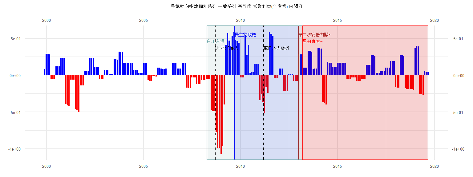
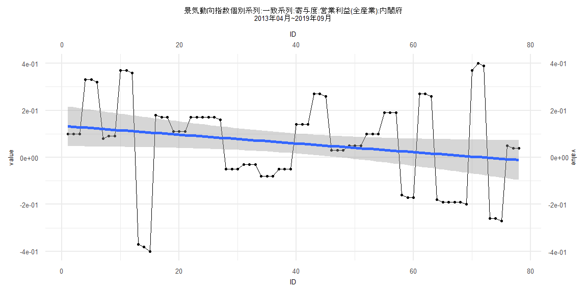
[1] "景気動向指数個別系列:一致系列:寄与度:営業利益(全産業):内閣府"
       Jan   Feb   Mar   Apr   May   Jun   Jul   Aug   Sep   Oct   Nov   Dec
1999                                                                    0.08
2000  0.29  0.29  0.28 -0.05 -0.05 -0.05  0.12  0.12  0.12  0.23  0.23  0.23
2001 -0.39 -0.41 -0.42 -0.06 -0.06 -0.06 -0.46 -0.47 -0.50 -0.14 -0.14 -0.14
2002  0.06  0.05  0.05  0.23  0.23  0.23  0.11  0.11  0.11 -0.05 -0.05 -0.05
2003  0.07  0.07  0.07  0.01  0.01  0.01  0.22  0.22  0.21  0.32  0.31  0.31
2004  0.16  0.16  0.16  0.16  0.16  0.16  0.07  0.07  0.07  0.03  0.03  0.03
2005  0.16  0.16  0.16 -0.07 -0.08 -0.08 -0.01 -0.01 -0.02  0.10  0.10  0.09
2006  0.08  0.08  0.09  0.00  0.00  0.00  0.17  0.17  0.17  0.09  0.09  0.09
2007  0.17  0.17  0.17 -0.17 -0.18 -0.18 -0.03 -0.03 -0.03 -0.12 -0.12 -0.12
2008 -0.07 -0.07 -0.07 -0.05 -0.05 -0.05 -0.47 -0.49 -0.49 -0.77 -0.99 -0.99
2009 -1.07 -0.96 -0.40  0.41  0.57  0.47  0.39  0.53  0.58  0.48  0.46  0.44
2010 -0.03 -0.03 -0.03  0.55  0.27  0.41  0.03  0.04  0.04  0.15  0.15  0.15
2011 -0.34 -0.26 -0.36 -0.52 -0.16 -0.24  0.59  0.56  0.53 -0.04 -0.04 -0.04
2012  0.09  0.09  0.09 -0.21 -0.21 -0.22  0.01  0.01  0.01 -0.08 -0.08 -0.08
2013  0.29  0.28  0.28  0.10  0.10  0.10  0.33  0.33  0.32  0.08  0.09  0.09
2014  0.37  0.37  0.36 -0.37 -0.38 -0.40  0.18  0.17  0.17  0.11  0.11  0.11
2015  0.17  0.17  0.17  0.17  0.17  0.16 -0.05 -0.05 -0.05 -0.03 -0.03 -0.03
2016 -0.08 -0.08 -0.08 -0.05 -0.05 -0.05  0.14  0.14  0.14  0.27  0.27  0.26
2017  0.03  0.03  0.03  0.05  0.05  0.05  0.10  0.10  0.10  0.19  0.19  0.19
2018 -0.16 -0.17 -0.17  0.27  0.27  0.26 -0.18 -0.19 -0.19 -0.19 -0.19 -0.20
2019  0.37  0.40  0.39 -0.26 -0.26 -0.27  0.05  0.04  0.04
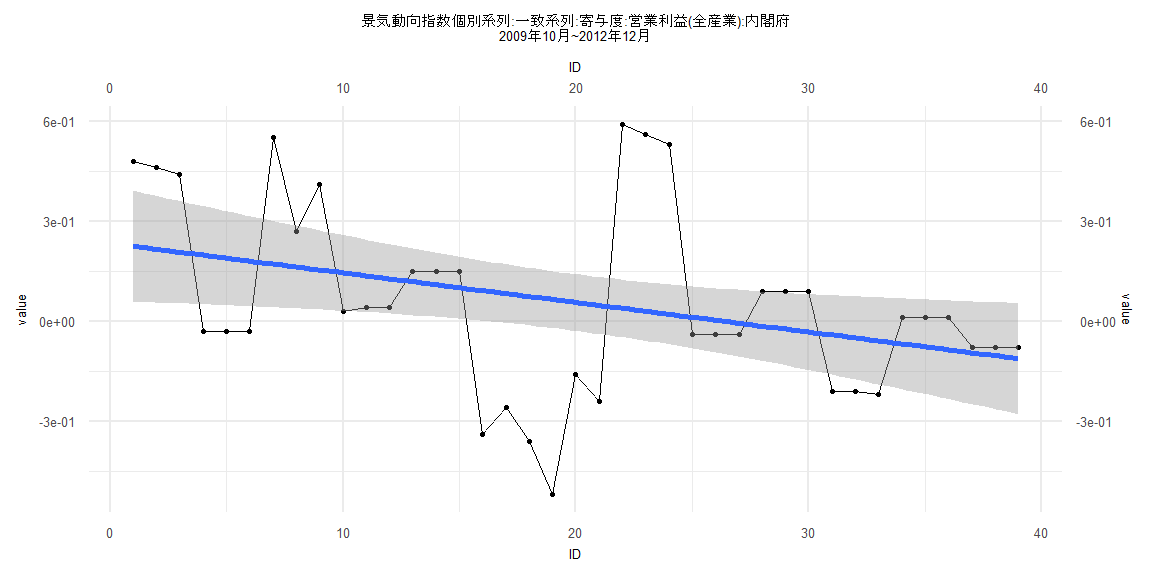
Call:
lm(formula = value ~ ID)

Residuals:
     Min       1Q   Median       3Q      Max
-0.58477 -0.16440  0.02384  0.11079  0.55185

Coefficients:
             Estimate Std. Error t value Pr(>|t|)
(Intercept)  0.233387   0.085494   2.730  0.00964 **
ID          -0.008874   0.003725  -2.382  0.02246 *
---
Signif. codes:  0 '***' 0.001 '**' 0.01 '*' 0.05 '.' 0.1 ' ' 1

Residual standard error: 0.2618 on 37 degrees of freedom
Multiple R-squared:  0.133, Adjusted R-squared:  0.1095
F-statistic: 5.675 on 1 and 37 DF,  p-value: 0.02246


    Two-sample Kolmogorov-Smirnov test

data:  lm_residuals and rnorm(n = length(lm_residuals), mean = 0, sd = sd(lm_residuals))
D = 0.28205, p-value = 0.08974
alternative hypothesis: two-sided


    Durbin-Watson test

data:  value ~ ID
DW = 0.94905, p-value = 0.00008276
alternative hypothesis: true autocorrelation is greater than 0


    studentized Breusch-Pagan test

data:  value ~ ID
BP = 0.84866, df = 1, p-value = 0.3569


    Box-Ljung test

data:  lm_residuals
X-squared = 11.048, df = 1, p-value = 0.0008879
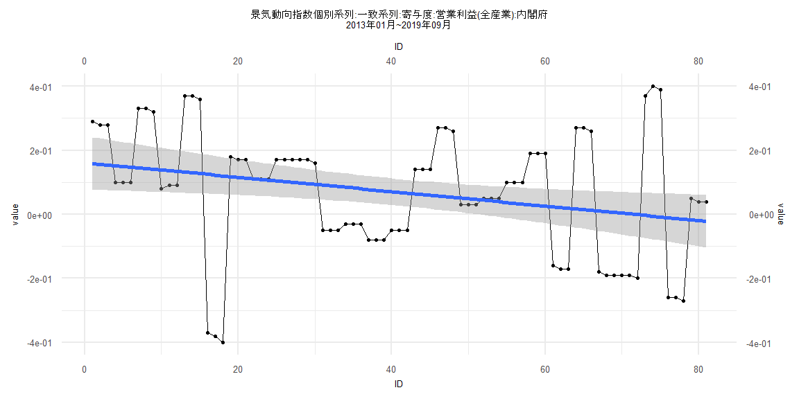
Call:
lm(formula = value ~ ID)

Residuals:
     Min       1Q   Median       3Q      Max
-0.52042 -0.13665  0.00837  0.12356  0.40565

Coefficients:
              Estimate Std. Error t value Pr(>|t|)
(Intercept)  0.1609475  0.0420976   3.823 0.000261 ***
ID          -0.0022514  0.0008919  -2.524 0.013603 *
---
Signif. codes:  0 '***' 0.001 '**' 0.01 '*' 0.05 '.' 0.1 ' ' 1

Residual standard error: 0.1877 on 79 degrees of freedom
Multiple R-squared:  0.07463,   Adjusted R-squared:  0.06292
F-statistic: 6.371 on 1 and 79 DF,  p-value: 0.0136


    Two-sample Kolmogorov-Smirnov test

data:  lm_residuals and rnorm(n = length(lm_residuals), mean = 0, sd = sd(lm_residuals))
D = 0.11111, p-value = 0.7027
alternative hypothesis: two-sided


    Durbin-Watson test

data:  value ~ ID
DW = 0.94296, p-value = 0.00000006081
alternative hypothesis: true autocorrelation is greater than 0


    studentized Breusch-Pagan test

data:  value ~ ID
BP = 0.49924, df = 1, p-value = 0.4798


    Box-Ljung test

data:  lm_residuals
X-squared = 23.14, df = 1, p-value = 0.000001506
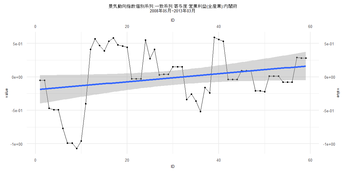
Call:
lm(formula = value ~ ID)

Residuals:
     Min       1Q   Median       3Q      Max
-0.93131 -0.27429  0.01273  0.23771  0.68469

Coefficients:
             Estimate Std. Error t value Pr(>|t|)
(Intercept) -0.192677   0.108411  -1.777   0.0809 .
ID           0.005999   0.003143   1.909   0.0613 .
---
Signif. codes:  0 '***' 0.001 '**' 0.01 '*' 0.05 '.' 0.1 ' ' 1

Residual standard error: 0.4111 on 57 degrees of freedom
Multiple R-squared:  0.06008,   Adjusted R-squared:  0.04359
F-statistic: 3.644 on 1 and 57 DF,  p-value: 0.06132


    Two-sample Kolmogorov-Smirnov test

data:  lm_residuals and rnorm(n = length(lm_residuals), mean = 0, sd = sd(lm_residuals))
D = 0.20339, p-value = 0.1748
alternative hypothesis: two-sided


    Durbin-Watson test

data:  value ~ ID
DW = 0.40649, p-value = 0.000000000000001197
alternative hypothesis: true autocorrelation is greater than 0


    studentized Breusch-Pagan test

data:  value ~ ID
BP = 15.583, df = 1, p-value = 0.00007895


    Box-Ljung test

data:  lm_residuals
X-squared = 39.223, df = 1, p-value = 0.000000000378
Call:
lm(formula = value ~ ID)

Residuals:
     Min       1Q   Median       3Q      Max
-0.50599 -0.12946  0.01124  0.08386  0.39825

Coefficients:
              Estimate Std. Error t value Pr(>|t|)
(Intercept)  0.1339061  0.0433096   3.092  0.00278 **
ID          -0.0018613  0.0009526  -1.954  0.05438 .
---
Signif. codes:  0 '***' 0.001 '**' 0.01 '*' 0.05 '.' 0.1 ' ' 1

Residual standard error: 0.1894 on 76 degrees of freedom
Multiple R-squared:  0.04783,   Adjusted R-squared:  0.03531
F-statistic: 3.818 on 1 and 76 DF,  p-value: 0.05438


    Two-sample Kolmogorov-Smirnov test

data:  lm_residuals and rnorm(n = length(lm_residuals), mean = 0, sd = sd(lm_residuals))
D = 0.11538, p-value = 0.6802
alternative hypothesis: two-sided


    Durbin-Watson test

data:  value ~ ID
DW = 0.95076, p-value = 0.0000001279
alternative hypothesis: true autocorrelation is greater than 0


    studentized Breusch-Pagan test

data:  value ~ ID
BP = 0.30791, df = 1, p-value = 0.579


    Box-Ljung test

data:  lm_residuals
X-squared = 22.247, df = 1, p-value = 0.000002397