Analysis
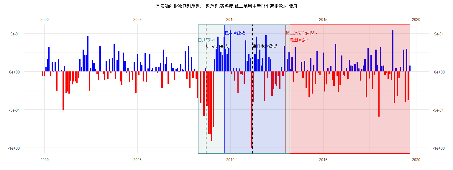
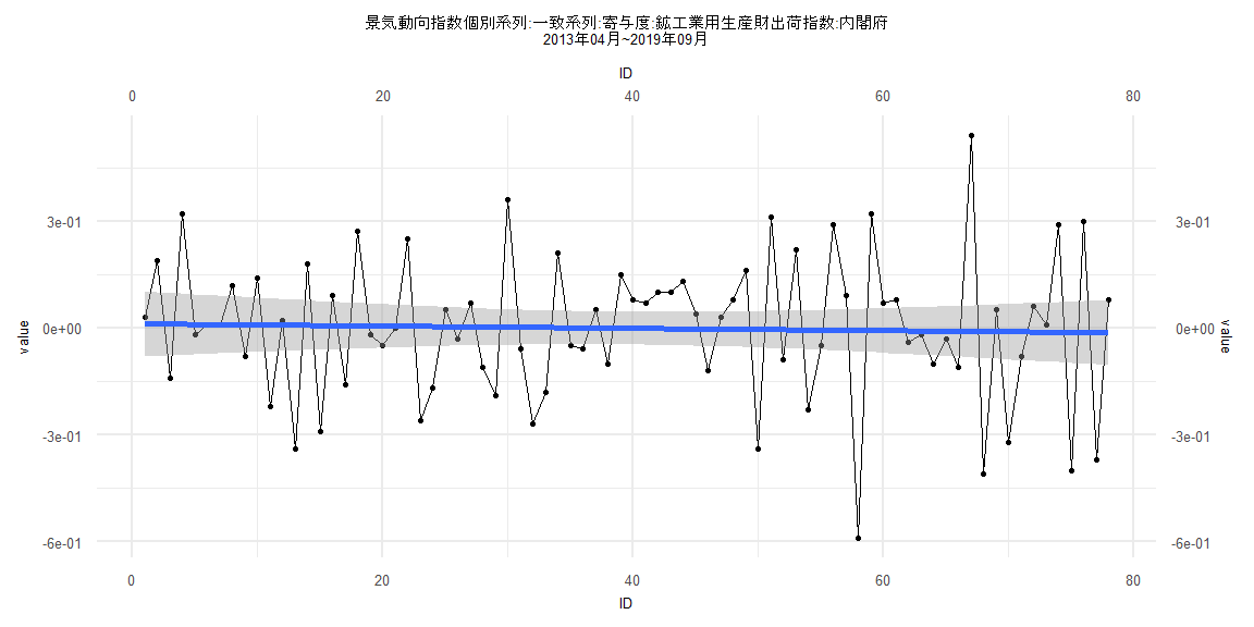
[1] "景気動向指数個別系列:一致系列:寄与度:鉱工業用生産財出荷指数:内閣府"
       Jan   Feb   Mar   Apr   May   Jun   Jul   Aug   Sep   Oct   Nov   Dec
1999                                                                   -0.06
2000 -0.06  0.06  0.17  0.32 -0.06  0.13 -0.01  0.13 -0.25  0.16  0.01  0.02
2001 -0.51  0.07 -0.28 -0.26 -0.29 -0.12 -0.17 -0.13 -0.13 -0.15 -0.08  0.16
2002  0.06  0.29  0.22  0.22  0.47 -0.25  0.05  0.15  0.11  0.03 -0.03 -0.11
2003  0.34  0.01 -0.03 -0.11  0.14 -0.10  0.16 -0.02  0.18  0.36 -0.10  0.15
2004  0.27 -0.13 -0.18  0.25  0.14 -0.02  0.05 -0.14 -0.01 -0.11  0.13 -0.28
2005  0.23 -0.05  0.12  0.09 -0.13  0.24 -0.14  0.04  0.23  0.02  0.05  0.01
2006  0.06 -0.02  0.06  0.11 -0.21  0.29  0.10  0.19 -0.16  0.00  0.11  0.05
2007 -0.11  0.03  0.05 -0.01  0.10  0.03  0.02  0.27 -0.10  0.33 -0.22  0.19
2008 -0.08  0.03 -0.10 -0.35  0.00 -0.41  0.01 -0.58  0.05 -0.45 -0.82 -0.82
2009 -0.91 -0.73  0.17  0.30  0.46  0.35  0.26  0.22  0.45  0.30  0.23  0.31
2010  0.54 -0.03  0.05 -0.12  0.05 -0.28  0.04 -0.03 -0.05 -0.16  0.41  0.14
2011  0.23  0.18 -1.00 -0.40  0.23  0.46  0.17  0.29  0.08  0.18 -0.38  0.48
2012 -0.08  0.19  0.17 -0.32 -0.23 -0.17 -0.19 -0.06 -0.23  0.06 -0.06  0.33
2013 -0.01  0.17  0.26  0.03  0.19 -0.14  0.32 -0.02  0.01  0.01  0.12 -0.08
2014  0.14 -0.22  0.02 -0.34  0.18 -0.29  0.09 -0.16  0.27 -0.02 -0.05  0.00
2015  0.25 -0.26 -0.17  0.05 -0.03  0.07 -0.11 -0.19  0.36 -0.06 -0.27 -0.18
2016  0.21 -0.05 -0.06  0.05 -0.10  0.15  0.08  0.07  0.10  0.10  0.13  0.04
2017 -0.12  0.03  0.08  0.16 -0.34  0.31 -0.09  0.22 -0.23 -0.05  0.29  0.09
2018 -0.59  0.32  0.07  0.08 -0.04 -0.02 -0.10 -0.03 -0.11  0.54 -0.41  0.05
2019 -0.32 -0.08  0.06  0.01  0.29 -0.40  0.30 -0.37  0.08
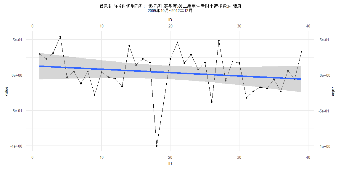
Call:
lm(formula = value ~ ID)

Residuals:
     Min       1Q   Median       3Q      Max
-1.04365 -0.14969 -0.00822  0.18021  0.47930

Coefficients:
             Estimate Std. Error t value Pr(>|t|)
(Intercept)  0.129528   0.095881   1.351    0.185
ID          -0.004771   0.004178  -1.142    0.261

Residual standard error: 0.2936 on 37 degrees of freedom
Multiple R-squared:  0.03405,   Adjusted R-squared:  0.007941
F-statistic: 1.304 on 1 and 37 DF,  p-value: 0.2608


    Two-sample Kolmogorov-Smirnov test

data:  lm_residuals and rnorm(n = length(lm_residuals), mean = 0, sd = sd(lm_residuals))
D = 0.10256, p-value = 0.9885
alternative hypothesis: two-sided


    Durbin-Watson test

data:  value ~ ID
DW = 1.7035, p-value = 0.1329
alternative hypothesis: true autocorrelation is greater than 0


    studentized Breusch-Pagan test

data:  value ~ ID
BP = 0.0087293, df = 1, p-value = 0.9256


    Box-Ljung test

data:  lm_residuals
X-squared = 0.60605, df = 1, p-value = 0.4363
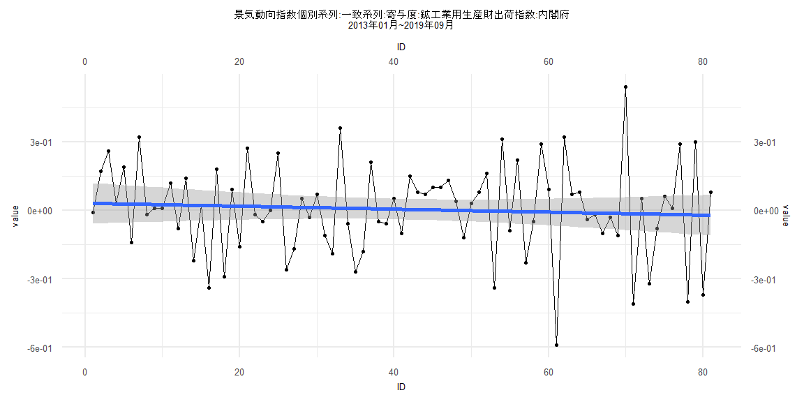
Call:
lm(formula = value ~ ID)

Residuals:
     Min       1Q   Median       3Q      Max
-0.58115 -0.10312 -0.00116  0.10190  0.55472

Coefficients:
              Estimate Std. Error t value Pr(>|t|)
(Intercept)  0.0309475  0.0455475   0.679    0.499
ID          -0.0006524  0.0009650  -0.676    0.501

Residual standard error: 0.2031 on 79 degrees of freedom
Multiple R-squared:  0.005753,  Adjusted R-squared:  -0.006833
F-statistic: 0.4571 on 1 and 79 DF,  p-value: 0.501


    Two-sample Kolmogorov-Smirnov test

data:  lm_residuals and rnorm(n = length(lm_residuals), mean = 0, sd = sd(lm_residuals))
D = 0.16049, p-value = 0.2488
alternative hypothesis: two-sided


    Durbin-Watson test

data:  value ~ ID
DW = 2.9014, p-value = 1
alternative hypothesis: true autocorrelation is greater than 0


    studentized Breusch-Pagan test

data:  value ~ ID
BP = 4.8274, df = 1, p-value = 0.02801


    Box-Ljung test

data:  lm_residuals
X-squared = 17.212, df = 1, p-value = 0.00003344
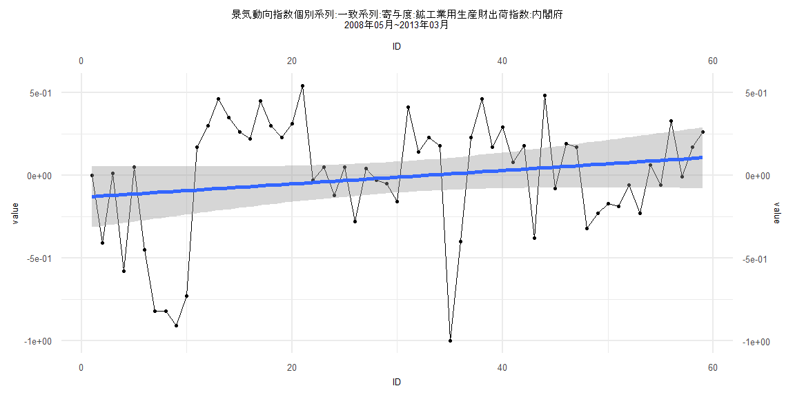
Call:
lm(formula = value ~ ID)

Residuals:
     Min       1Q   Median       3Q      Max
-1.00840 -0.24556  0.08213  0.24768  0.58834

Coefficients:
             Estimate Std. Error t value Pr(>|t|)
(Intercept) -0.133442   0.094653  -1.410    0.164
ID           0.004053   0.002744   1.477    0.145

Residual standard error: 0.3589 on 57 degrees of freedom
Multiple R-squared:  0.03686,   Adjusted R-squared:  0.01996
F-statistic: 2.181 on 1 and 57 DF,  p-value: 0.1452


    Two-sample Kolmogorov-Smirnov test

data:  lm_residuals and rnorm(n = length(lm_residuals), mean = 0, sd = sd(lm_residuals))
D = 0.084746, p-value = 0.9854
alternative hypothesis: two-sided


    Durbin-Watson test

data:  value ~ ID
DW = 1.0971, p-value = 0.0000644
alternative hypothesis: true autocorrelation is greater than 0


    studentized Breusch-Pagan test

data:  value ~ ID
BP = 5.3148, df = 1, p-value = 0.02115


    Box-Ljung test

data:  lm_residuals
X-squared = 12.492, df = 1, p-value = 0.0004086
Call:
lm(formula = value ~ ID)

Residuals:
     Min       1Q   Median       3Q      Max
-0.58305 -0.10023  0.00642  0.10207  0.54983

Coefficients:
              Estimate Std. Error t value Pr(>|t|)
(Intercept)  0.0116217  0.0467511   0.249    0.804
ID          -0.0003202  0.0010283  -0.311    0.756

Residual standard error: 0.2045 on 76 degrees of freedom
Multiple R-squared:  0.001274,  Adjusted R-squared:  -0.01187
F-statistic: 0.09696 on 1 and 76 DF,  p-value: 0.7564


    Two-sample Kolmogorov-Smirnov test

data:  lm_residuals and rnorm(n = length(lm_residuals), mean = 0, sd = sd(lm_residuals))
D = 0.076923, p-value = 0.9766
alternative hypothesis: two-sided


    Durbin-Watson test

data:  value ~ ID
DW = 2.9455, p-value = 1
alternative hypothesis: true autocorrelation is greater than 0


    studentized Breusch-Pagan test

data:  value ~ ID
BP = 4.6272, df = 1, p-value = 0.03147


    Box-Ljung test

data:  lm_residuals
X-squared = 18.22, df = 1, p-value = 0.00001968