Analysis
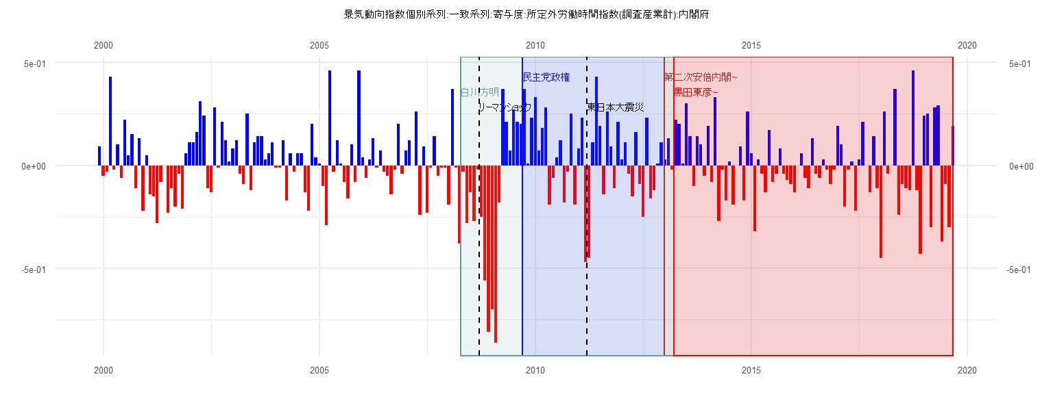
[1] "景気動向指数個別系列:一致系列:寄与度:所定外労働時間指数(調査産業計):内閣府"
       Jan   Feb   Mar   Apr   May   Jun   Jul   Aug   Sep   Oct   Nov   Dec
1999                                                                    0.09
2000 -0.05 -0.03  0.43 -0.02  0.10 -0.06  0.22  0.05  0.15 -0.11  0.13 -0.22
2001  0.05 -0.14 -0.15 -0.28 -0.08  0.00 -0.23 -0.11 -0.20 -0.04 -0.21  0.06
2002  0.11  0.11  0.16  0.31  0.24 -0.11 -0.13  0.28 -0.01  0.21  0.12  0.02
2003  0.08  0.12 -0.04 -0.09  0.25 -0.12  0.11  0.14  0.14  0.03  0.06  0.11
2004 -0.01 -0.01  0.12 -0.17  0.06 -0.03  0.06  0.06 -0.13 -0.22  0.20  0.04
2005  0.01 -0.10 -0.29  0.46 -0.03  0.12  0.01 -0.08 -0.16  0.10 -0.08  0.46
2006  0.04 -0.06  0.03  0.13 -0.01  0.07 -0.03 -0.05 -0.14 -0.02  0.20 -0.04
2007  0.07  0.12  0.00  0.26 -0.24  0.09 -0.23 -0.01  0.14 -0.05 -0.01 -0.01
2008 -0.19  0.37 -0.01 -0.38 -0.03 -0.28 -0.13 -0.27 -0.02 -0.25 -0.56 -0.81
2009 -0.70 -0.86 -0.18  0.37  0.21  0.07  0.27  0.21  0.20  0.37  0.01  0.23
2010  0.33  0.07  0.18  0.28 -0.19 -0.06  0.04  0.12 -0.18 -0.03  0.25 -0.19
2011  0.08  0.23 -0.47 -0.45  0.11  0.43  0.19 -0.14  0.26  0.09 -0.11  0.21
2012  0.03  0.11 -0.04 -0.15  0.16 -0.09 -0.25  0.23 -0.16 -0.12  0.01  0.11
2013  0.03  0.13 -0.02  0.22  0.20  0.01  0.30  0.14 -0.10  0.14  0.10 -0.05
2014  0.19 -0.08  0.33 -0.27 -0.02 -0.17  0.02 -0.19  0.00  0.09 -0.17  0.26
2015  0.06 -0.32  0.03 -0.04 -0.13  0.17 -0.08 -0.04  0.08 -0.04 -0.07 -0.09
2016 -0.13  0.00  0.06 -0.06 -0.11  0.13 -0.04 -0.06  0.03 -0.02 -0.09 -0.02
2017  0.19  0.10 -0.20 -0.02  0.02 -0.22  0.03  0.21  0.00 -0.13  0.14 -0.11
2018 -0.45  0.26 -0.04  0.00  0.37 -0.24 -0.09 -0.11 -0.12  0.46 -0.12 -0.43
2019  0.24  0.25 -0.30  0.28  0.29 -0.37 -0.09 -0.30  0.19
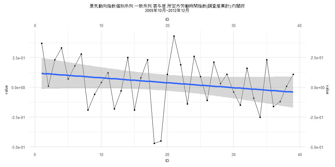
Call:
lm(formula = value ~ ID)

Residuals:
    Min      1Q  Median      3Q     Max
-0.5167 -0.1280  0.0250  0.1655  0.3957

Coefficients:
             Estimate Std. Error t value Pr(>|t|)
(Intercept)  0.121174   0.067166   1.804   0.0794 .
ID          -0.004136   0.002927  -1.413   0.1660
---
Signif. codes:  0 '***' 0.001 '**' 0.01 '*' 0.05 '.' 0.1 ' ' 1

Residual standard error: 0.2057 on 37 degrees of freedom
Multiple R-squared:  0.0512,    Adjusted R-squared:  0.02556
F-statistic: 1.997 on 1 and 37 DF,  p-value: 0.166


    Two-sample Kolmogorov-Smirnov test

data:  lm_residuals and rnorm(n = length(lm_residuals), mean = 0, sd = sd(lm_residuals))
D = 0.12821, p-value = 0.9114
alternative hypothesis: two-sided


    Durbin-Watson test

data:  value ~ ID
DW = 1.9693, p-value = 0.3939
alternative hypothesis: true autocorrelation is greater than 0


    studentized Breusch-Pagan test

data:  value ~ ID
BP = 0.2193, df = 1, p-value = 0.6396


    Box-Ljung test

data:  lm_residuals
X-squared = 0.0063251, df = 1, p-value = 0.9366
Call:
lm(formula = value ~ ID)

Residuals:
     Min       1Q   Median       3Q      Max
-0.43034 -0.09247 -0.01837  0.10885  0.48851

Coefficients:
              Estimate Std. Error t value Pr(>|t|)
(Intercept)  0.0403056  0.0410491   0.982    0.329
ID          -0.0009831  0.0008697  -1.130    0.262

Residual standard error: 0.183 on 79 degrees of freedom
Multiple R-squared:  0.01592,   Adjusted R-squared:  0.003458
F-statistic: 1.278 on 1 and 79 DF,  p-value: 0.2618


    Two-sample Kolmogorov-Smirnov test

data:  lm_residuals and rnorm(n = length(lm_residuals), mean = 0, sd = sd(lm_residuals))
D = 0.098765, p-value = 0.8277
alternative hypothesis: two-sided


    Durbin-Watson test

data:  value ~ ID
DW = 2.4831, p-value = 0.9821
alternative hypothesis: true autocorrelation is greater than 0


    studentized Breusch-Pagan test

data:  value ~ ID
BP = 10.032, df = 1, p-value = 0.001538


    Box-Ljung test

data:  lm_residuals
X-squared = 5.3165, df = 1, p-value = 0.02113
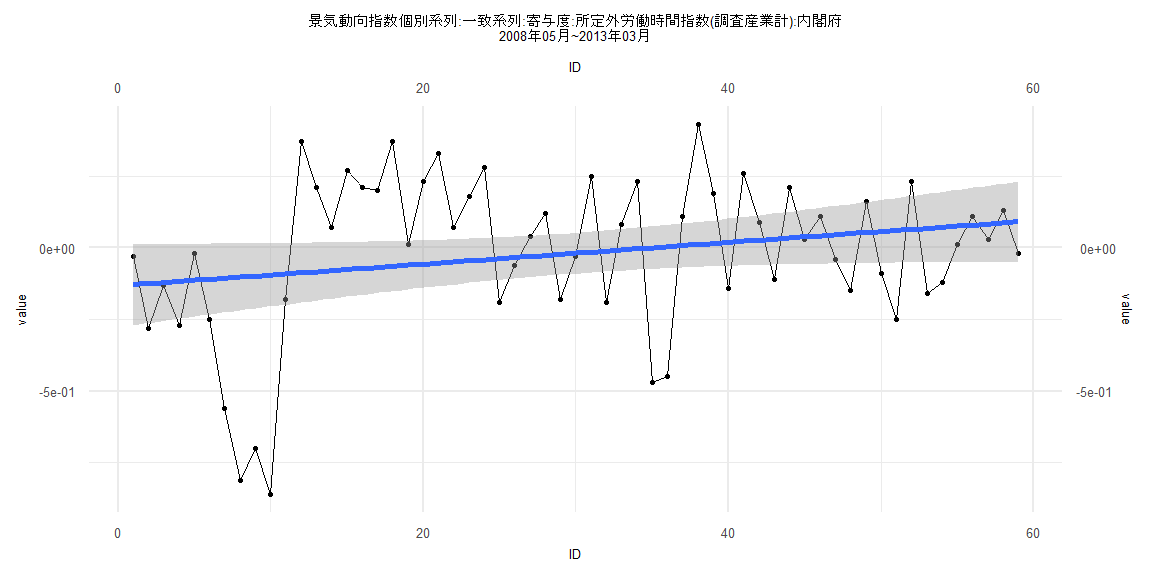
Call:
lm(formula = value ~ ID)

Residuals:
     Min       1Q   Median       3Q      Max
-0.76532 -0.15235  0.04301  0.17546  0.45711

Coefficients:
             Estimate Std. Error t value Pr(>|t|)
(Intercept) -0.132531   0.072149  -1.837   0.0714 .
ID           0.003785   0.002092   1.810   0.0756 .
---
Signif. codes:  0 '***' 0.001 '**' 0.01 '*' 0.05 '.' 0.1 ' ' 1

Residual standard error: 0.2736 on 57 degrees of freedom
Multiple R-squared:  0.05433,   Adjusted R-squared:  0.03774
F-statistic: 3.275 on 1 and 57 DF,  p-value: 0.07562


    Two-sample Kolmogorov-Smirnov test

data:  lm_residuals and rnorm(n = length(lm_residuals), mean = 0, sd = sd(lm_residuals))
D = 0.084746, p-value = 0.9854
alternative hypothesis: two-sided


    Durbin-Watson test

data:  value ~ ID
DW = 1.0368, p-value = 0.00001979
alternative hypothesis: true autocorrelation is greater than 0


    studentized Breusch-Pagan test

data:  value ~ ID
BP = 7.0489, df = 1, p-value = 0.007931


    Box-Ljung test

data:  lm_residuals
X-squared = 14.238, df = 1, p-value = 0.0001611
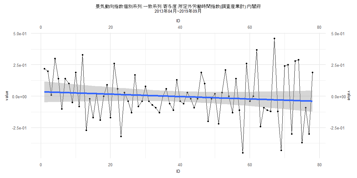
Call:
lm(formula = value ~ ID)

Residuals:
     Min       1Q   Median       3Q      Max
-0.43051 -0.09403 -0.01868  0.11028  0.48809

Coefficients:
              Estimate Std. Error t value Pr(>|t|)
(Intercept)  0.0359774  0.0425686   0.845    0.401
ID          -0.0009563  0.0009363  -1.021    0.310

Residual standard error: 0.1862 on 76 degrees of freedom
Multiple R-squared:  0.01354,   Adjusted R-squared:  0.0005601
F-statistic: 1.043 on 1 and 76 DF,  p-value: 0.3103


    Two-sample Kolmogorov-Smirnov test

data:  lm_residuals and rnorm(n = length(lm_residuals), mean = 0, sd = sd(lm_residuals))
D = 0.14103, p-value = 0.4221
alternative hypothesis: two-sided


    Durbin-Watson test

data:  value ~ ID
DW = 2.4599, p-value = 0.9743
alternative hypothesis: true autocorrelation is greater than 0


    studentized Breusch-Pagan test

data:  value ~ ID
BP = 8.6254, df = 1, p-value = 0.003315


    Box-Ljung test

data:  lm_residuals
X-squared = 4.9192, df = 1, p-value = 0.02656