Analysis
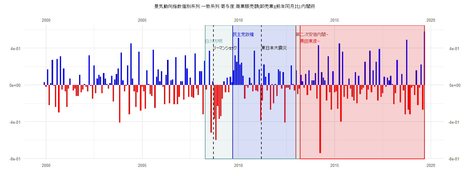
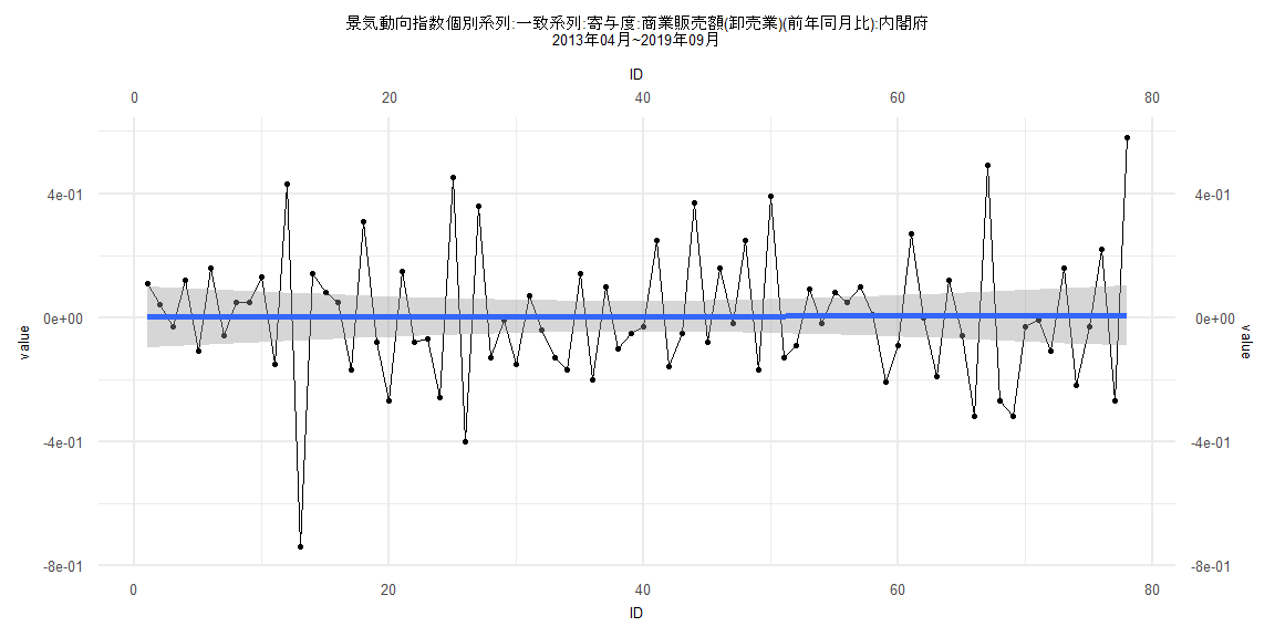
[1] "景気動向指数個別系列:一致系列:寄与度:商業販売額(卸売業)(前年同月比):内閣府"
       Jan   Feb   Mar   Apr   May   Jun   Jul   Aug   Sep   Oct   Nov   Dec
1999                                                                    0.03
2000 -0.02  0.17 -0.22  0.02  0.27 -0.01 -0.24  0.28 -0.30  0.31 -0.05  0.18
2001 -0.07 -0.24 -0.04  0.07  0.00 -0.06 -0.04 -0.12 -0.12  0.11 -0.08 -0.05
2002  0.01 -0.02 -0.07  0.32 -0.01 -0.15  0.21 -0.09  0.07  0.11  0.09 -0.09
2003  0.13  0.07  0.01 -0.04  0.02  0.10 -0.18  0.06  0.12  0.18 -0.41  0.35
2004  0.05 -0.07 -0.01  0.21 -0.32  0.45  0.07 -0.07 -0.24 -0.08  0.36 -0.28
2005 -0.02 -0.07 -0.26  0.16  0.01 -0.10 -0.12  0.38 -0.25  0.09  0.17  0.04
2006  0.15 -0.02 -0.21  0.11  0.27 -0.20  0.05  0.06 -0.21  0.30 -0.21 -0.13
2007  0.04  0.04 -0.16  0.32  0.18 -0.13  0.08 -0.13 -0.14  0.34 -0.04 -0.11
2008  0.15  0.15 -0.32  0.26 -0.05  0.00  0.37 -0.52  0.04 -0.37 -0.60 -0.23
2009 -0.37 -0.34 -0.15  0.04 -0.08  0.08 -0.08  0.09  0.03  0.16  0.32  0.25
2010  0.51  0.22  0.24  0.10 -0.15 -0.01 -0.03  0.08  0.02 -0.07  0.37 -0.06
2011 -0.07  0.17 -0.39 -0.17  0.22  0.09 -0.06  0.13 -0.27  0.01 -0.20  0.01
2012 -0.12  0.17  0.15 -0.04  0.14 -0.41 -0.03 -0.03 -0.05  0.21  0.01 -0.06
2013  0.16 -0.10 -0.04  0.11  0.04 -0.03  0.12 -0.11  0.16 -0.06  0.05  0.05
2014  0.13 -0.15  0.43 -0.74  0.14  0.08  0.05 -0.17  0.31 -0.08 -0.27  0.15
2015 -0.08 -0.07 -0.26  0.45 -0.40  0.36 -0.13 -0.01 -0.15  0.07 -0.04 -0.13
2016 -0.17  0.14 -0.20  0.10 -0.10 -0.05 -0.03  0.25 -0.16 -0.05  0.37 -0.08
2017  0.16 -0.02  0.25 -0.17  0.39 -0.13 -0.09  0.09 -0.02  0.08  0.05  0.10
2018  0.01 -0.21 -0.09  0.27  0.00 -0.19  0.12 -0.06 -0.32  0.49 -0.27 -0.32
2019 -0.03 -0.01 -0.11  0.16 -0.22 -0.03  0.22 -0.27  0.58
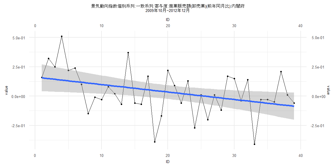
Call:
lm(formula = value ~ ID)

Residuals:
     Min       1Q   Median       3Q      Max
-0.43760 -0.12077  0.01693  0.11513  0.37333

Coefficients:
             Estimate Std. Error t value Pr(>|t|)
(Intercept)  0.162119   0.058974   2.749  0.00919 **
ID          -0.006362   0.002570  -2.476  0.01799 *
---
Signif. codes:  0 '***' 0.001 '**' 0.01 '*' 0.05 '.' 0.1 ' ' 1

Residual standard error: 0.1806 on 37 degrees of freedom
Multiple R-squared:  0.1421,    Adjusted R-squared:  0.1189
F-statistic:  6.13 on 1 and 37 DF,  p-value: 0.01799


    Two-sample Kolmogorov-Smirnov test

data:  lm_residuals and rnorm(n = length(lm_residuals), mean = 0, sd = sd(lm_residuals))
D = 0.23077, p-value = 0.2523
alternative hypothesis: two-sided


    Durbin-Watson test

data:  value ~ ID
DW = 1.9796, p-value = 0.4064
alternative hypothesis: true autocorrelation is greater than 0


    studentized Breusch-Pagan test

data:  value ~ ID
BP = 0.05916, df = 1, p-value = 0.8078


    Box-Ljung test

data:  lm_residuals
X-squared = 0.0041516, df = 1, p-value = 0.9486
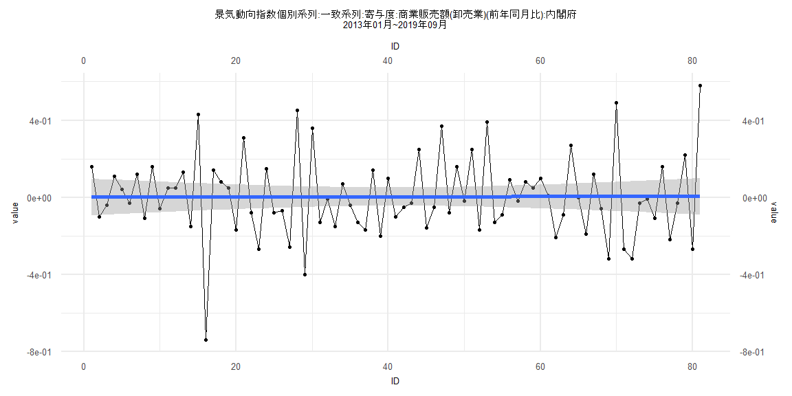
Call:
lm(formula = value ~ ID)

Residuals:
     Min       1Q   Median       3Q      Max
-0.74239 -0.13296 -0.03201  0.11795  0.57516

Coefficients:
              Estimate Std. Error t value Pr(>|t|)
(Intercept) 0.00178704 0.04843025   0.037    0.971
ID          0.00003771 0.00102610   0.037    0.971

Residual standard error: 0.2159 on 79 degrees of freedom
Multiple R-squared:  1.71e-05,  Adjusted R-squared:  -0.01264
F-statistic: 0.001351 on 1 and 79 DF,  p-value: 0.9708


    Two-sample Kolmogorov-Smirnov test

data:  lm_residuals and rnorm(n = length(lm_residuals), mean = 0, sd = sd(lm_residuals))
D = 0.12346, p-value = 0.5705
alternative hypothesis: two-sided


    Durbin-Watson test

data:  value ~ ID
DW = 2.9437, p-value = 1
alternative hypothesis: true autocorrelation is greater than 0


    studentized Breusch-Pagan test

data:  value ~ ID
BP = 0.27853, df = 1, p-value = 0.5977


    Box-Ljung test

data:  lm_residuals
X-squared = 22.736, df = 1, p-value = 0.000001858
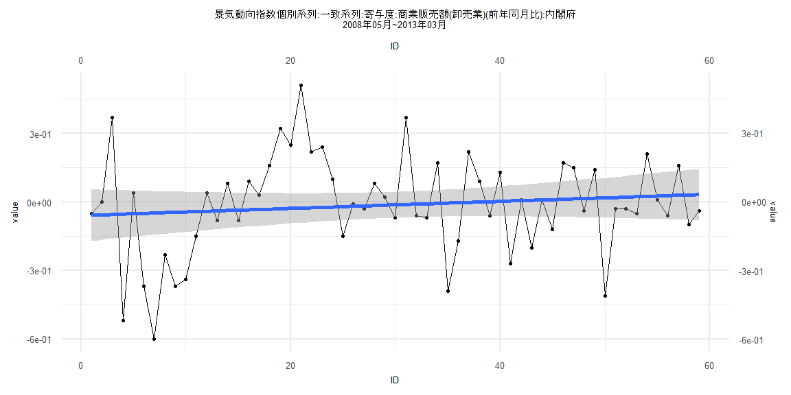
Call:
lm(formula = value ~ ID)

Residuals:
     Min       1Q   Median       3Q      Max
-0.55150 -0.09754  0.00120  0.12598  0.53682

Coefficients:
             Estimate Std. Error t value Pr(>|t|)
(Intercept) -0.059345   0.057469  -1.033    0.306
ID           0.001549   0.001666   0.930    0.356

Residual standard error: 0.2179 on 57 degrees of freedom
Multiple R-squared:  0.01494,   Adjusted R-squared:  -0.002345
F-statistic: 0.8643 on 1 and 57 DF,  p-value: 0.3565


    Two-sample Kolmogorov-Smirnov test

data:  lm_residuals and rnorm(n = length(lm_residuals), mean = 0, sd = sd(lm_residuals))
D = 0.15254, p-value = 0.5021
alternative hypothesis: two-sided


    Durbin-Watson test

data:  value ~ ID
DW = 1.5964, p-value = 0.04341
alternative hypothesis: true autocorrelation is greater than 0


    studentized Breusch-Pagan test

data:  value ~ ID
BP = 5.6635, df = 1, p-value = 0.01732


    Box-Ljung test

data:  lm_residuals
X-squared = 2.5031, df = 1, p-value = 0.1136
Call:
lm(formula = value ~ ID)

Residuals:
     Min       1Q   Median       3Q      Max
-0.74168 -0.13276 -0.02757  0.11797  0.57458

Coefficients:
              Estimate Std. Error t value Pr(>|t|)
(Intercept) 0.00093240 0.05008086   0.019    0.985
ID          0.00005754 0.00110150   0.052    0.958

Residual standard error: 0.219 on 76 degrees of freedom
Multiple R-squared:  3.59e-05,  Adjusted R-squared:  -0.01312
F-statistic: 0.002729 on 1 and 76 DF,  p-value: 0.9585


    Two-sample Kolmogorov-Smirnov test

data:  lm_residuals and rnorm(n = length(lm_residuals), mean = 0, sd = sd(lm_residuals))
D = 0.16667, p-value = 0.2297
alternative hypothesis: two-sided


    Durbin-Watson test

data:  value ~ ID
DW = 2.948, p-value = 1
alternative hypothesis: true autocorrelation is greater than 0


    studentized Breusch-Pagan test

data:  value ~ ID
BP = 0.094819, df = 1, p-value = 0.7581


    Box-Ljung test

data:  lm_residuals
X-squared = 21.988, df = 1, p-value = 0.000002743