Analysis
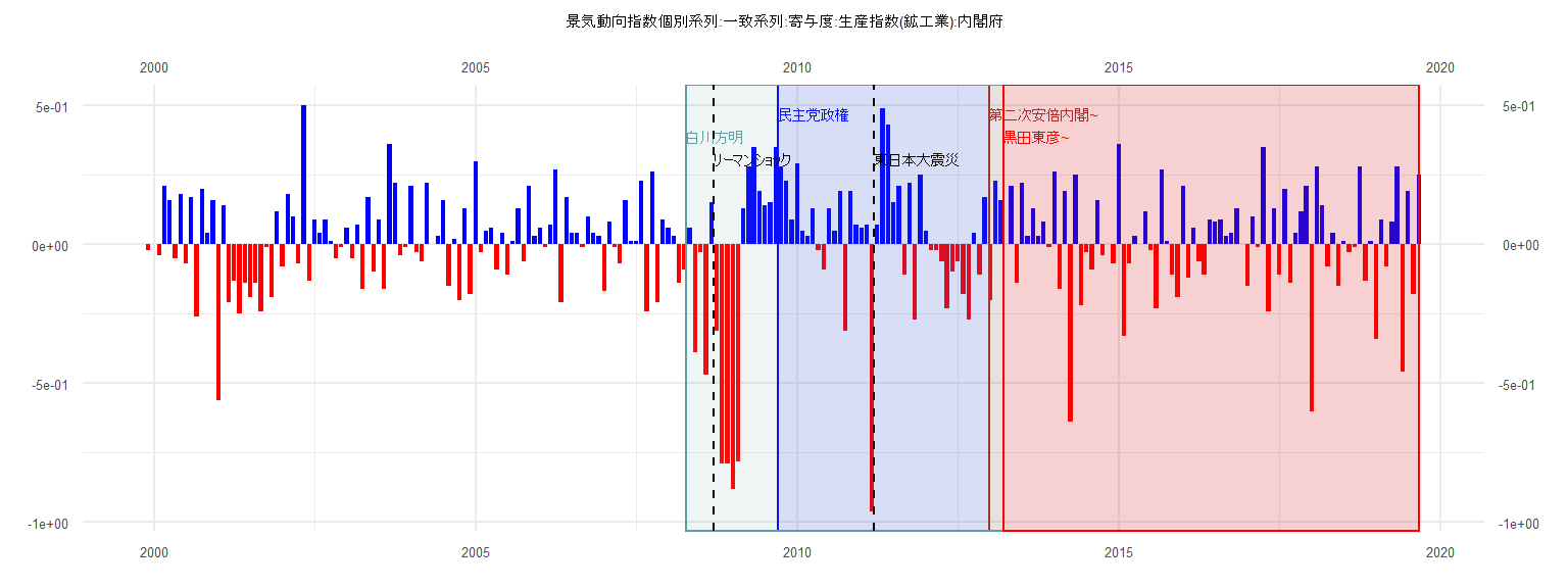
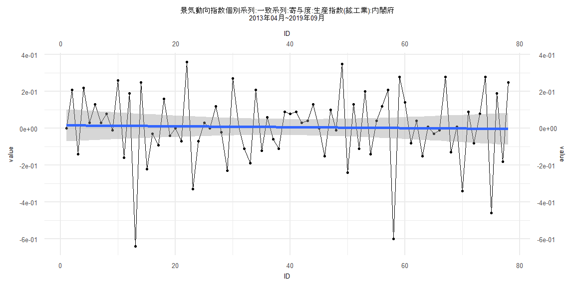
[1] "景気動向指数個別系列:一致系列:寄与度:生産指数(鉱工業):内閣府"
       Jan   Feb   Mar   Apr   May   Jun   Jul   Aug   Sep   Oct   Nov   Dec
1999                                                                   -0.02
2000  0.00 -0.04  0.21  0.16 -0.05  0.18 -0.07  0.17 -0.26  0.20  0.04  0.16
2001 -0.56  0.14 -0.21 -0.13 -0.25 -0.14 -0.19 -0.14 -0.24 -0.01 -0.19  0.12
2002 -0.08  0.18  0.10 -0.07  0.50 -0.13  0.09  0.04  0.09  0.01 -0.05 -0.01
2003  0.06 -0.05  0.07 -0.16  0.17 -0.10  0.09 -0.16  0.36  0.22 -0.04 -0.01
2004  0.21 -0.03 -0.06  0.22  0.00  0.03  0.16 -0.15  0.02 -0.20  0.13 -0.18
2005  0.30 -0.03  0.05  0.06 -0.09  0.04 -0.11  0.01  0.13 -0.06  0.21  0.03
2006  0.06 -0.01  0.07  0.27 -0.21  0.17  0.04  0.04 -0.01  0.10  0.04  0.03
2007 -0.17  0.08 -0.01 -0.07  0.16  0.01  0.01  0.23 -0.24  0.26 -0.21  0.09
2008  0.06  0.03 -0.14 -0.09  0.06 -0.39 -0.03 -0.47  0.15 -0.31 -0.79 -0.79
2009 -0.88 -0.78  0.13  0.28  0.35  0.19  0.14  0.15  0.35  0.28  0.23  0.09
2010  0.29  0.05  0.03  0.13 -0.02 -0.09  0.13  0.05  0.19 -0.31  0.19  0.07
2011  0.06  0.07 -0.96  0.07  0.49  0.43  0.15  0.21 -0.11  0.22 -0.27  0.25
2012  0.05 -0.02 -0.02 -0.06 -0.23 -0.10 -0.06 -0.18 -0.27  0.04 -0.11  0.17
2013 -0.20  0.23  0.16  0.00  0.21 -0.14  0.22  0.03  0.13  0.03  0.08 -0.01
2014  0.26 -0.16  0.19 -0.64  0.25 -0.22 -0.03 -0.09  0.16 -0.04  0.00 -0.07
2015  0.36 -0.33 -0.07  0.03  0.00  0.12 -0.02 -0.23  0.27  0.01 -0.11 -0.19
2016  0.21 -0.12  0.06 -0.06 -0.11  0.09  0.08  0.09  0.03  0.04  0.13  0.00
2017 -0.15  0.10 -0.01  0.35 -0.24  0.13 -0.11  0.20 -0.14  0.04  0.12  0.21
2018 -0.60  0.28  0.14 -0.08  0.04 -0.15  0.01 -0.03 -0.01  0.28 -0.13  0.01
2019 -0.34  0.09 -0.08  0.08  0.28 -0.46  0.19 -0.18  0.25
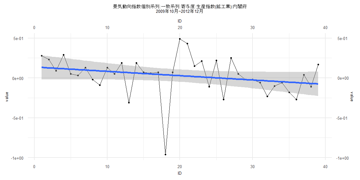
Call:
lm(formula = value ~ ID)

Residuals:
     Min       1Q   Median       3Q      Max
-0.99988 -0.06802  0.00922  0.12287  0.46103

Coefficients:
             Estimate Std. Error t value Pr(>|t|)
(Intercept)  0.138003   0.077957   1.770   0.0849 .
ID          -0.005451   0.003397  -1.605   0.1170
---
Signif. codes:  0 '***' 0.001 '**' 0.01 '*' 0.05 '.' 0.1 ' ' 1

Residual standard error: 0.2388 on 37 degrees of freedom
Multiple R-squared:  0.06508,   Adjusted R-squared:  0.03981
F-statistic: 2.575 on 1 and 37 DF,  p-value: 0.117


    Two-sample Kolmogorov-Smirnov test

data:  lm_residuals and rnorm(n = length(lm_residuals), mean = 0, sd = sd(lm_residuals))
D = 0.10256, p-value = 0.9885
alternative hypothesis: two-sided


    Durbin-Watson test

data:  value ~ ID
DW = 1.9749, p-value = 0.4008
alternative hypothesis: true autocorrelation is greater than 0


    studentized Breusch-Pagan test

data:  value ~ ID
BP = 0.0032552, df = 1, p-value = 0.9545


    Box-Ljung test

data:  lm_residuals
X-squared = 0.0019474, df = 1, p-value = 0.9648
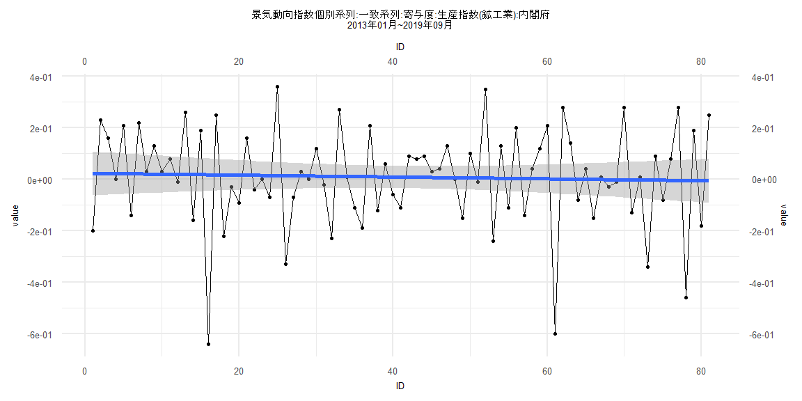
Call:
lm(formula = value ~ ID)

Residuals:
     Min       1Q   Median       3Q      Max
-0.65790 -0.11384  0.00994  0.12580  0.34534

Coefficients:
              Estimate Std. Error t value Pr(>|t|)
(Intercept)  0.0236667  0.0436464   0.542    0.589
ID          -0.0003604  0.0009247  -0.390    0.698

Residual standard error: 0.1946 on 79 degrees of freedom
Multiple R-squared:  0.001919,  Adjusted R-squared:  -0.01071
F-statistic: 0.1519 on 1 and 79 DF,  p-value: 0.6978


    Two-sample Kolmogorov-Smirnov test

data:  lm_residuals and rnorm(n = length(lm_residuals), mean = 0, sd = sd(lm_residuals))
D = 0.18519, p-value = 0.1245
alternative hypothesis: two-sided


    Durbin-Watson test

data:  value ~ ID
DW = 2.9799, p-value = 1
alternative hypothesis: true autocorrelation is greater than 0


    studentized Breusch-Pagan test

data:  value ~ ID
BP = 0.19956, df = 1, p-value = 0.6551


    Box-Ljung test

data:  lm_residuals
X-squared = 21.79, df = 1, p-value = 0.000003042
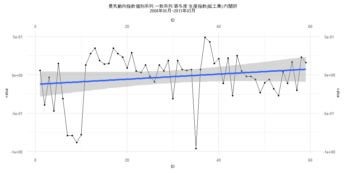
Call:
lm(formula = value ~ ID)

Residuals:
     Min       1Q   Median       3Q      Max
-0.95427 -0.15750  0.07906  0.21067  0.48908

Coefficients:
             Estimate Std. Error t value Pr(>|t|)
(Intercept) -0.122209   0.083643  -1.461    0.149
ID           0.003328   0.002425   1.372    0.175

Residual standard error: 0.3172 on 57 degrees of freedom
Multiple R-squared:  0.03199,   Adjusted R-squared:  0.01501
F-statistic: 1.884 on 1 and 57 DF,  p-value: 0.1753


    Two-sample Kolmogorov-Smirnov test

data:  lm_residuals and rnorm(n = length(lm_residuals), mean = 0, sd = sd(lm_residuals))
D = 0.30508, p-value = 0.00792
alternative hypothesis: two-sided


    Durbin-Watson test

data:  value ~ ID
DW = 1.1844, p-value = 0.0002969
alternative hypothesis: true autocorrelation is greater than 0


    studentized Breusch-Pagan test

data:  value ~ ID
BP = 4.8126, df = 1, p-value = 0.02825


    Box-Ljung test

data:  lm_residuals
X-squared = 10.147, df = 1, p-value = 0.001446
Call:
lm(formula = value ~ ID)

Residuals:
     Min       1Q   Median       3Q      Max
-0.65330 -0.11087  0.00983  0.12255  0.34891

Coefficients:
              Estimate Std. Error t value Pr(>|t|)
(Intercept)  0.0164902  0.0445036   0.371    0.712
ID          -0.0002455  0.0009788  -0.251    0.803

Residual standard error: 0.1946 on 76 degrees of freedom
Multiple R-squared:  0.0008267, Adjusted R-squared:  -0.01232
F-statistic: 0.06288 on 1 and 76 DF,  p-value: 0.8027


    Two-sample Kolmogorov-Smirnov test

data:  lm_residuals and rnorm(n = length(lm_residuals), mean = 0, sd = sd(lm_residuals))
D = 0.15385, p-value = 0.316
alternative hypothesis: two-sided


    Durbin-Watson test

data:  value ~ ID
DW = 3.0213, p-value = 1
alternative hypothesis: true autocorrelation is greater than 0


    studentized Breusch-Pagan test

data:  value ~ ID
BP = 0.21986, df = 1, p-value = 0.6391


    Box-Ljung test

data:  lm_residuals
X-squared = 22.063, df = 1, p-value = 0.000002639