Analysis
[1] "景気動向指数個別系列:一致系列:寄与度:耐久消費財出荷指数:内閣府"
Jan Feb Mar Apr May Jun Jul Aug Sep Oct Nov Dec
1999 -0.05
2000 -0.06 0.11 0.04 0.30 -0.15 0.16 -0.12 0.10 -0.10 0.05 0.01 0.21
2001 -0.43 0.26 0.04 -0.08 -0.10 0.05 0.01 0.04 -0.20 0.14 -0.31 -0.10
2002 0.16 0.13 -0.06 0.02 0.33 -0.22 0.02 0.12 0.09 -0.04 0.29 -0.25
2003 0.03 -0.06 -0.13 0.16 -0.02 0.01 -0.04 0.05 0.19 0.05 -0.07 0.12
2004 0.03 -0.09 0.00 -0.02 0.11 -0.02 0.34 -0.49 0.18 0.05 0.12 -0.19
2005 -0.01 0.12 0.02 0.36 -0.40 0.15 0.01 -0.10 0.22 0.01 -0.04 0.19
2006 0.12 -0.02 0.18 0.29 -0.22 -0.07 0.10 0.07 -0.03 -0.01 0.26 -0.06
2007 0.03 0.02 -0.02 0.03 0.11 0.16 -0.45 0.38 -0.34 0.16 -0.02 0.17
2008 0.10 -0.10 -0.01 0.05 -0.13 -0.36 -0.03 -0.29 -0.05 -0.27 -0.41 -0.60
2009 -0.99 -0.34 0.02 -0.01 0.49 0.18 -0.09 0.07 0.29 0.25 0.22 0.02
2010 0.22 0.13 0.08 -0.11 -0.30 -0.04 -0.10 0.18 0.11 -0.20 0.17 0.00
2011 -0.20 0.18 -1.10 -0.53 0.57 0.52 0.18 0.04 0.07 0.29 -0.58 0.57
2012 0.22 0.10 -0.25 -0.17 -0.33 -0.38 -0.03 0.01 -0.46 -0.13 -0.23 0.42
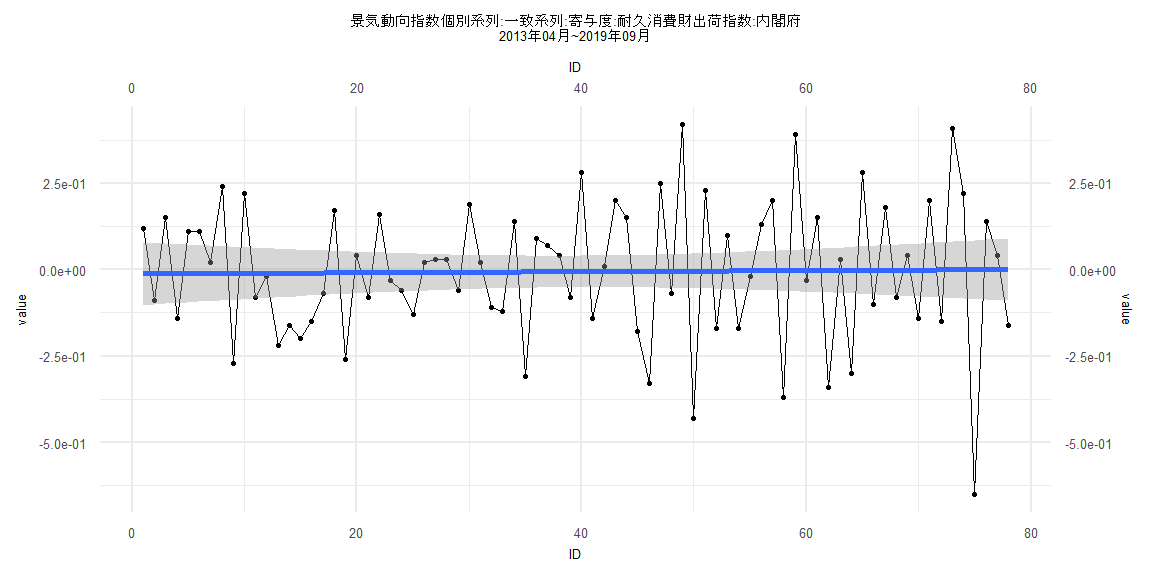
2013 0.19 0.11 -0.06 0.12 -0.09 0.15 -0.14 0.11 0.11 0.02 0.24 -0.27
2014 0.22 -0.08 -0.02 -0.22 -0.16 -0.20 -0.15 -0.07 0.17 -0.26 0.04 -0.08
2015 0.16 -0.03 -0.06 -0.13 0.02 0.03 0.03 -0.06 0.19 0.02 -0.11 -0.12
2016 0.14 -0.31 0.09 0.07 0.04 -0.08 0.28 -0.14 0.01 0.20 0.15 -0.18
2017 -0.33 0.25 -0.07 0.42 -0.43 0.23 -0.17 0.10 -0.17 -0.02 0.13 0.20
2018 -0.37 0.39 -0.03 0.15 -0.34 0.03 -0.30 0.28 -0.10 0.18 -0.08 0.04
2019 -0.14 0.20 -0.15 0.41 0.22 -0.65 0.14 0.04 -0.16
Call:
lm(formula = value ~ ID)

Residuals:
     Min       1Q   Median       3Q      Max
-1.09365 -0.17145  0.04654  0.16188  0.61583

Coefficients:
             Estimate Std. Error t value Pr(>|t|)
(Intercept)  0.072605   0.108836   0.667    0.509
ID          -0.004387   0.004742  -0.925    0.361

Residual standard error: 0.3333 on 37 degrees of freedom
Multiple R-squared:  0.0226,    Adjusted R-squared:  -0.003815
F-statistic: 0.8556 on 1 and 37 DF,  p-value: 0.361


    Two-sample Kolmogorov-Smirnov test

data:  lm_residuals and rnorm(n = length(lm_residuals), mean = 0, sd = sd(lm_residuals))
D = 0.12821, p-value = 0.9114
alternative hypothesis: two-sided


    Durbin-Watson test

data:  value ~ ID
DW = 1.7969, p-value = 0.2077
alternative hypothesis: true autocorrelation is greater than 0


    studentized Breusch-Pagan test

data:  value ~ ID
BP = 0.41938, df = 1, p-value = 0.5172


    Box-Ljung test

data:  lm_residuals
X-squared = 0.17701, df = 1, p-value = 0.674
Call:
lm(formula = value ~ ID)

Residuals:
     Min       1Q   Median       3Q      Max
-0.64406 -0.13451  0.01979  0.14942  0.42359

Coefficients:
               Estimate  Std. Error t value Pr(>|t|)
(Intercept)  0.00112037  0.04477671   0.025    0.980
ID          -0.00009056  0.00094870  -0.095    0.924

Residual standard error: 0.1996 on 79 degrees of freedom
Multiple R-squared:  0.0001153, Adjusted R-squared:  -0.01254
F-statistic: 0.009112 on 1 and 79 DF,  p-value: 0.9242


    Two-sample Kolmogorov-Smirnov test

data:  lm_residuals and rnorm(n = length(lm_residuals), mean = 0, sd = sd(lm_residuals))
D = 0.12346, p-value = 0.5705
alternative hypothesis: two-sided


    Durbin-Watson test

data:  value ~ ID
DW = 2.8689, p-value = 1
alternative hypothesis: true autocorrelation is greater than 0


    studentized Breusch-Pagan test

data:  value ~ ID
BP = 7.6231, df = 1, p-value = 0.005762


    Box-Ljung test

data:  lm_residuals
X-squared = 16.558, df = 1, p-value = 0.00004719
Call:
lm(formula = value ~ ID)

Residuals:
     Min       1Q   Median       3Q      Max
-1.06480 -0.17060  0.06175  0.21020  0.59982

Coefficients:
             Estimate Std. Error t value Pr(>|t|)
(Intercept) -0.129316   0.087705  -1.474    0.146
ID           0.002689   0.002542   1.058    0.295

Residual standard error: 0.3326 on 57 degrees of freedom
Multiple R-squared:  0.01925,   Adjusted R-squared:  0.002042
F-statistic: 1.119 on 1 and 57 DF,  p-value: 0.2947


    Two-sample Kolmogorov-Smirnov test

data:  lm_residuals and rnorm(n = length(lm_residuals), mean = 0, sd = sd(lm_residuals))
D = 0.15254, p-value = 0.5021
alternative hypothesis: two-sided


    Durbin-Watson test

data:  value ~ ID
DW = 1.4377, p-value = 0.009272
alternative hypothesis: true autocorrelation is greater than 0


    studentized Breusch-Pagan test

data:  value ~ ID
BP = 0.002346, df = 1, p-value = 0.9614


    Box-Ljung test

data:  lm_residuals
X-squared = 4.8827, df = 1, p-value = 0.02713
Call:
lm(formula = value ~ ID)

Residuals:
     Min       1Q   Median       3Q      Max
-0.64986 -0.13300  0.02125  0.15093  0.42426

Coefficients:
              Estimate Std. Error t value Pr(>|t|)
(Intercept) -0.0120380  0.0461338  -0.261    0.795
ID           0.0001587  0.0010147   0.156    0.876

Residual standard error: 0.2018 on 76 degrees of freedom
Multiple R-squared:  0.0003218, Adjusted R-squared:  -0.01283
F-statistic: 0.02446 on 1 and 76 DF,  p-value: 0.8761


    Two-sample Kolmogorov-Smirnov test

data:  lm_residuals and rnorm(n = length(lm_residuals), mean = 0, sd = sd(lm_residuals))
D = 0.11538, p-value = 0.6802
alternative hypothesis: two-sided


    Durbin-Watson test

data:  value ~ ID
DW = 2.8976, p-value = 1
alternative hypothesis: true autocorrelation is greater than 0


    studentized Breusch-Pagan test

data:  value ~ ID
BP = 7.0072, df = 1, p-value = 0.008118


    Box-Ljung test

data:  lm_residuals
X-squared = 16.833, df = 1, p-value = 0.00004081