Analysis
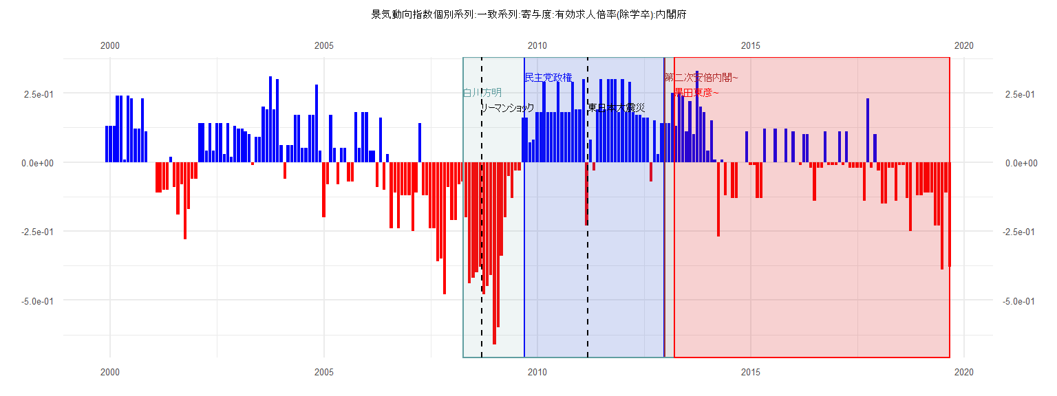
[1] "景気動向指数個別系列:一致系列:寄与度:有効求人倍率(除学卒):内閣府"
       Jan   Feb   Mar   Apr   May   Jun   Jul   Aug   Sep   Oct   Nov   Dec
1999                                                                    0.13
2000  0.13  0.13  0.24  0.24  0.01  0.24  0.23  0.12  0.12  0.23  0.11  0.00
2001  0.00 -0.11 -0.11 -0.10 -0.10  0.02 -0.09 -0.19 -0.08 -0.28 -0.17 -0.06
2002 -0.06  0.14  0.14  0.04  0.14  0.04  0.14  0.14  0.03  0.14  0.02  0.13
2003  0.12  0.12  0.11  0.10 -0.01  0.09  0.09  0.20  0.19  0.31  0.19  0.30
2004  0.06 -0.06  0.06  0.06  0.17  0.17  0.05  0.05  0.17  0.17  0.28  0.04
2005 -0.20 -0.08  0.17  0.05 -0.08  0.05  0.05 -0.07 -0.07  0.18  0.05  0.18
2006  0.18  0.04  0.04 -0.09  0.16 -0.10  0.03 -0.24 -0.11 -0.24 -0.12 -0.12
2007 -0.12 -0.25 -0.11  0.14 -0.12 -0.12 -0.24 -0.24 -0.36 -0.35 -0.48 -0.09
2008 -0.21 -0.21 -0.08 -0.07 -0.20 -0.44 -0.42 -0.40 -0.38 -0.48 -0.45 -0.41
2009 -0.66 -0.60 -0.34 -0.20 -0.05 -0.13 -0.03 -0.03  0.16  0.16  0.07  0.08
2010  0.18  0.18  0.29  0.18  0.18  0.18  0.29  0.18  0.18  0.18  0.29  0.19
2011  0.19  0.30 -0.23  0.08 -0.03  0.19  0.30  0.19  0.30  0.30  0.30  0.18
2012  0.30  0.18  0.29  0.18  0.17  0.17  0.16  0.16 -0.07  0.15  0.03  0.14
2013  0.14  0.14  0.25  0.13  0.25  0.24  0.11  0.22  0.10  0.33  0.20  0.18
2014  0.04  0.15  0.01 -0.27  0.01 -0.12  0.00 -0.13 -0.13  0.00  0.00  0.11
2015 -0.01 -0.01 -0.13 -0.13  0.12  0.00  0.00  0.12  0.00  0.00  0.12  0.00
2016  0.11  0.00 -0.01  0.10  0.10 -0.02 -0.14 -0.02 -0.02  0.11 -0.01 -0.01
2017 -0.01  0.11 -0.01  0.11 -0.02 -0.02 -0.02 -0.02 -0.14  0.23 -0.02  0.10
2018 -0.03 -0.15 -0.15 -0.02 -0.02 -0.14 -0.01 -0.01 -0.13 -0.25  0.00 -0.12
2019 -0.12 -0.11 -0.11 -0.11 -0.23 -0.23 -0.39 -0.11 -0.38
Call:
lm(formula = value ~ ID)

Residuals:
     Min       1Q   Median       3Q      Max
-0.40421 -0.00747  0.00232  0.06336  0.13273

Coefficients:
              Estimate Std. Error t value  Pr(>|t|)
(Intercept)  0.1867072  0.0365651   5.106 0.0000102 ***
ID          -0.0006943  0.0015933  -0.436     0.666
---
Signif. codes:  0 '***' 0.001 '**' 0.01 '*' 0.05 '.' 0.1 ' ' 1

Residual standard error: 0.112 on 37 degrees of freedom
Multiple R-squared:  0.005106,  Adjusted R-squared:  -0.02178
F-statistic: 0.1899 on 1 and 37 DF,  p-value: 0.6655


    Two-sample Kolmogorov-Smirnov test

data:  lm_residuals and rnorm(n = length(lm_residuals), mean = 0, sd = sd(lm_residuals))
D = 0.17949, p-value = 0.5622
alternative hypothesis: two-sided


    Durbin-Watson test

data:  value ~ ID
DW = 1.6594, p-value = 0.1048
alternative hypothesis: true autocorrelation is greater than 0


    studentized Breusch-Pagan test

data:  value ~ ID
BP = 0.09328, df = 1, p-value = 0.76


    Box-Ljung test

data:  lm_residuals
X-squared = 1.2038, df = 1, p-value = 0.2726
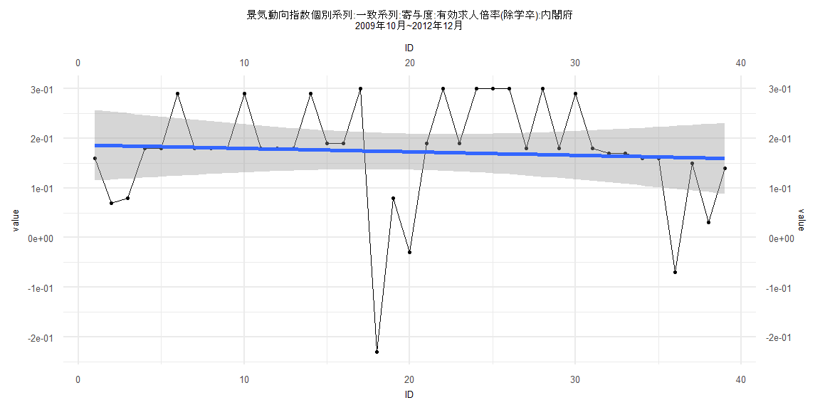
Call:
lm(formula = value ~ ID)

Residuals:
     Min       1Q   Median       3Q      Max
-0.35647 -0.06122  0.00024  0.07910  0.29502

Coefficients:
              Estimate Std. Error t value      Pr(>|t|)
(Intercept)  0.1441852  0.0245648    5.87 0.00000009777 ***
ID          -0.0036070  0.0005205   -6.93 0.00000000101 ***
---
Signif. codes:  0 '***' 0.001 '**' 0.01 '*' 0.05 '.' 0.1 ' ' 1

Residual standard error: 0.1095 on 79 degrees of freedom
Multiple R-squared:  0.3781,    Adjusted R-squared:  0.3702
F-statistic: 48.03 on 1 and 79 DF,  p-value: 0.000000001015


    Two-sample Kolmogorov-Smirnov test

data:  lm_residuals and rnorm(n = length(lm_residuals), mean = 0, sd = sd(lm_residuals))
D = 0.11111, p-value = 0.7027
alternative hypothesis: two-sided


    Durbin-Watson test

data:  value ~ ID
DW = 1.4524, p-value = 0.004171
alternative hypothesis: true autocorrelation is greater than 0


    studentized Breusch-Pagan test

data:  value ~ ID
BP = 0.15457, df = 1, p-value = 0.6942


    Box-Ljung test

data:  lm_residuals
X-squared = 5.0598, df = 1, p-value = 0.02449
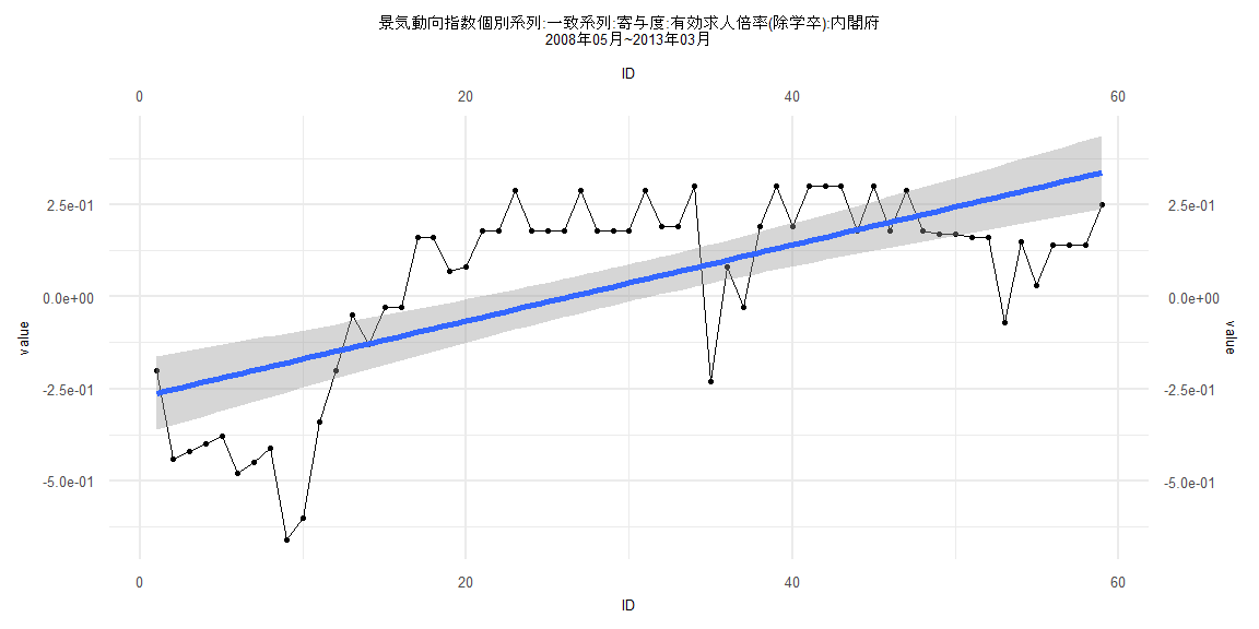
Call:
lm(formula = value ~ ID)

Residuals:
     Min       1Q   Median       3Q      Max
-0.48072 -0.16262  0.04933  0.14754  0.32479

Coefficients:
             Estimate Std. Error t value      Pr(>|t|)
(Intercept) -0.272168   0.051111  -5.325 0.00000177792 ***
ID           0.010321   0.001482   6.966 0.00000000363 ***
---
Signif. codes:  0 '***' 0.001 '**' 0.01 '*' 0.05 '.' 0.1 ' ' 1

Residual standard error: 0.1938 on 57 degrees of freedom
Multiple R-squared:  0.4598,    Adjusted R-squared:  0.4504
F-statistic: 48.52 on 1 and 57 DF,  p-value: 0.000000003627


    Two-sample Kolmogorov-Smirnov test

data:  lm_residuals and rnorm(n = length(lm_residuals), mean = 0, sd = sd(lm_residuals))
D = 0.16949, p-value = 0.3674
alternative hypothesis: two-sided


    Durbin-Watson test

data:  value ~ ID
DW = 0.50379, p-value = 0.0000000000004203
alternative hypothesis: true autocorrelation is greater than 0


    studentized Breusch-Pagan test

data:  value ~ ID
BP = 4.0019, df = 1, p-value = 0.04545


    Box-Ljung test

data:  lm_residuals
X-squared = 34.482, df = 1, p-value = 0.000000004301
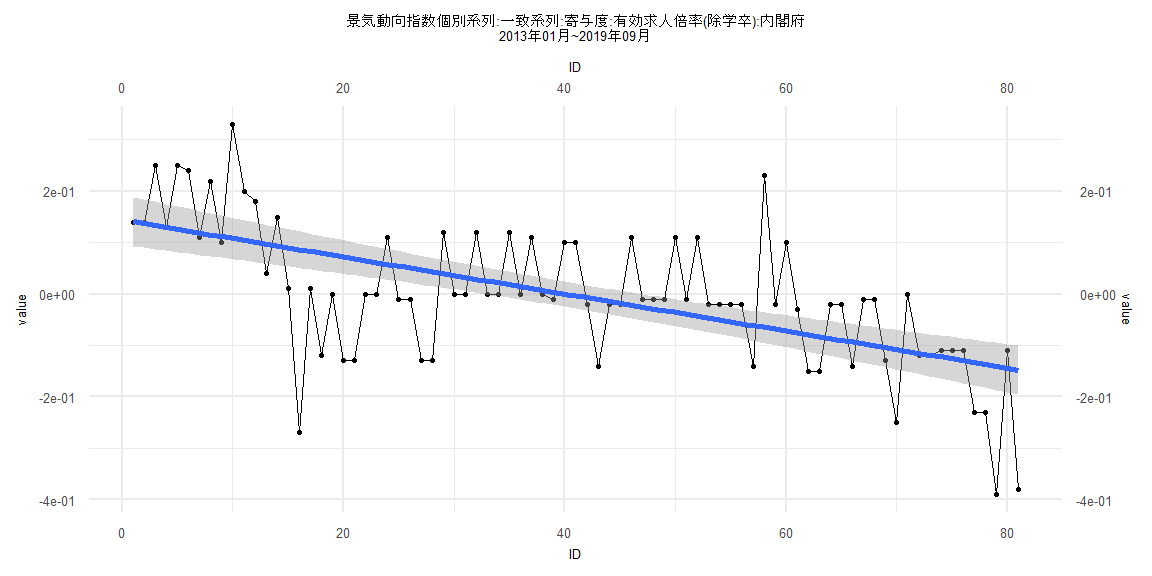
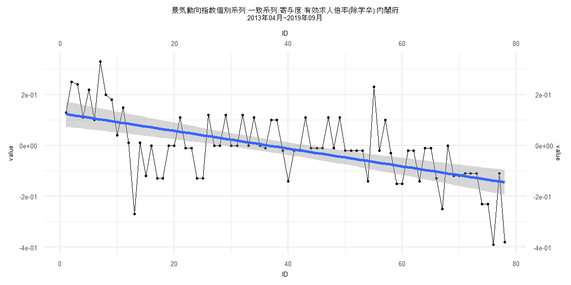
Call:
lm(formula = value ~ ID)

Residuals:
     Min       1Q   Median       3Q      Max
-0.35179 -0.05964  0.00286  0.07994  0.29471

Coefficients:
              Estimate Std. Error t value    Pr(>|t|)
(Intercept)  0.1271362  0.0253371   5.018 0.000003344 ***
ID          -0.0034880  0.0005573  -6.259 0.000000021 ***
---
Signif. codes:  0 '***' 0.001 '**' 0.01 '*' 0.05 '.' 0.1 ' ' 1

Residual standard error: 0.1108 on 76 degrees of freedom
Multiple R-squared:  0.3401,    Adjusted R-squared:  0.3315
F-statistic: 39.18 on 1 and 76 DF,  p-value: 0.00000002105


    Two-sample Kolmogorov-Smirnov test

data:  lm_residuals and rnorm(n = length(lm_residuals), mean = 0, sd = sd(lm_residuals))
D = 0.089744, p-value = 0.9147
alternative hypothesis: two-sided


    Durbin-Watson test

data:  value ~ ID
DW = 1.4465, p-value = 0.004375
alternative hypothesis: true autocorrelation is greater than 0


    studentized Breusch-Pagan test

data:  value ~ ID
BP = 0.35679, df = 1, p-value = 0.5503


    Box-Ljung test

data:  lm_residuals
X-squared = 4.9494, df = 1, p-value = 0.0261