Analysis
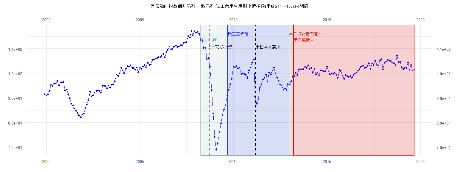
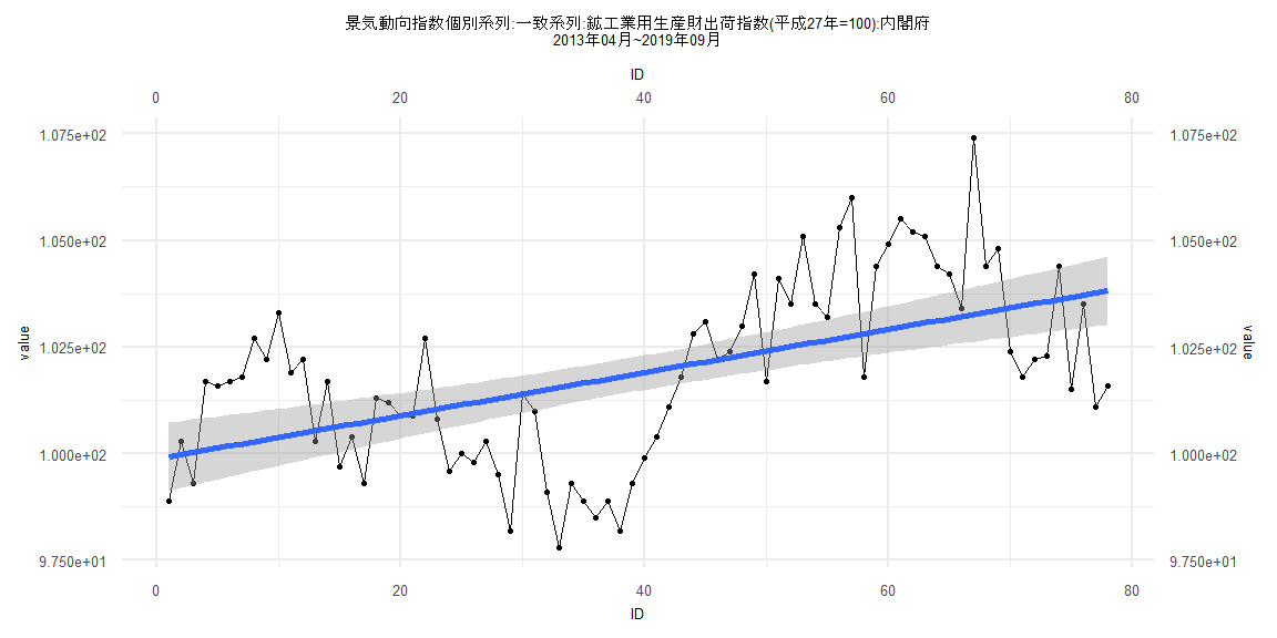
[1] "景気動向指数個別系列:一致系列:鉱工業用生産財出荷指数(平成27年=100):内閣府"
       Jan   Feb   Mar   Apr   May   Jun   Jul   Aug   Sep   Oct   Nov   Dec
1999                                                                    91.5
2000  91.1  91.6  92.9  95.3  94.9  95.9  95.9  96.9  95.1  96.3  96.4  96.6
2001  93.0  93.5  91.5  89.7  87.7  86.9  85.7  84.8  83.9  82.8  82.2  83.3
2002  83.7  85.8  87.4  89.0  92.5  90.6  91.0  92.1  92.9  93.1  92.9  92.1
2003  94.9  95.0  94.8  94.0  95.1  94.4  95.6  95.5  96.9  99.6  98.9 100.1
2004 102.2 101.3 100.0 101.9 103.0 102.9 103.3 102.3 102.3 101.5 102.5 100.5
2005 102.2 101.9 102.8 103.5 102.6 104.4 103.4 103.7 105.5 105.7 106.1 106.2
2006 106.7 106.6 107.1 108.0 106.5 108.7 109.5 111.0 109.9 110.0 110.9 111.4
2007 110.7 111.0 111.5 111.5 112.3 112.6 112.8 115.3 114.6 117.3 115.6 117.2
2008 116.6 116.9 116.2 113.5 113.6 110.4 110.5 105.9 106.3 102.7  93.3  83.8
2009  74.2  69.0  71.6  76.0  79.8  83.1  85.2  87.0  91.0  93.5  95.4  98.0
2010 102.8 102.6 103.0 102.0 102.4  99.7 100.0  99.8  99.4  98.1 101.3 102.4
2011 104.3 105.8  90.7  87.7  89.4  94.1  95.4  97.6  98.2  99.6  96.7 100.3
2012  99.7 101.1 102.4 100.0  98.3  97.0  95.6  95.1  93.4  93.8  93.3  95.7
2013  95.6  96.8  98.7  98.9 100.3  99.3 101.7 101.6 101.7 101.8 102.7 102.2
2014 103.3 101.9 102.2 100.3 101.7  99.7 100.4  99.3 101.3 101.2 100.9 100.9
2015 102.7 100.8  99.6 100.0  99.8 100.3  99.5  98.2 101.4 101.0  99.1  97.8
2016  99.3  98.9  98.5  98.9  98.2  99.3  99.9 100.4 101.1 101.8 102.8 103.1
2017 102.2 102.4 103.0 104.2 101.7 104.1 103.5 105.1 103.5 103.2 105.3 106.0
2018 101.8 104.4 104.9 105.5 105.2 105.1 104.4 104.2 103.4 107.4 104.4 104.8
2019 102.4 101.8 102.2 102.3 104.4 101.5 103.5 101.1 101.6
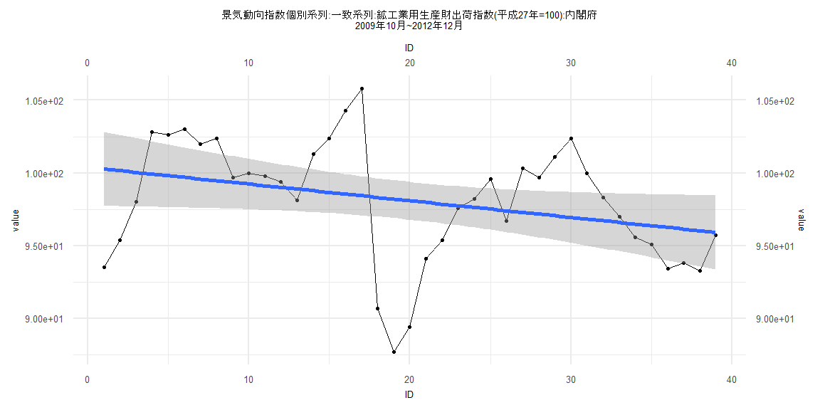
Call:
lm(formula = value ~ ID)

Residuals:
     Min       1Q   Median       3Q      Max
-10.5069  -2.1923   0.3974   2.8315   7.3639

Coefficients:
             Estimate Std. Error t value            Pr(>|t|)
(Intercept) 100.38421    1.30562  76.886 <0.0000000000000002 ***
ID           -0.11460    0.05689  -2.014              0.0513 .
---
Signif. codes:  0 '***' 0.001 '**' 0.01 '*' 0.05 '.' 0.1 ' ' 1

Residual standard error: 3.999 on 37 degrees of freedom
Multiple R-squared:  0.09882,   Adjusted R-squared:  0.07446
F-statistic: 4.057 on 1 and 37 DF,  p-value: 0.05129


    Two-sample Kolmogorov-Smirnov test

data:  lm_residuals and rnorm(n = length(lm_residuals), mean = 0, sd = sd(lm_residuals))
D = 0.17949, p-value = 0.5622
alternative hypothesis: two-sided


    Durbin-Watson test

data:  value ~ ID
DW = 0.64264, p-value = 0.0000001304
alternative hypothesis: true autocorrelation is greater than 0


    studentized Breusch-Pagan test

data:  value ~ ID
BP = 0.75197, df = 1, p-value = 0.3859


    Box-Ljung test

data:  lm_residuals
X-squared = 17.231, df = 1, p-value = 0.00003311
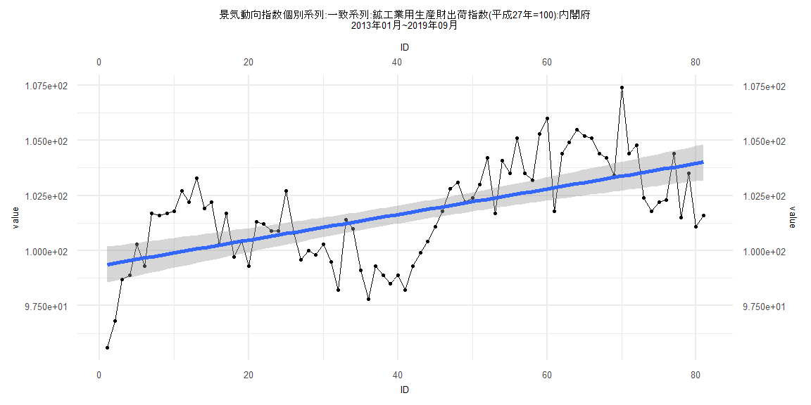
Call:
lm(formula = value ~ ID)

Residuals:
    Min      1Q  Median      3Q     Max
-3.7765 -1.2835  0.0819  1.4877  4.0239

Coefficients:
             Estimate Std. Error t value             Pr(>|t|)
(Intercept) 99.318488   0.413534 240.170 < 0.0000000000000002 ***
ID           0.057965   0.008762   6.616        0.00000000402 ***
---
Signif. codes:  0 '***' 0.001 '**' 0.01 '*' 0.05 '.' 0.1 ' ' 1

Residual standard error: 1.844 on 79 degrees of freedom
Multiple R-squared:  0.3565,    Adjusted R-squared:  0.3484
F-statistic: 43.77 on 1 and 79 DF,  p-value: 0.000000004016


    Two-sample Kolmogorov-Smirnov test

data:  lm_residuals and rnorm(n = length(lm_residuals), mean = 0, sd = sd(lm_residuals))
D = 0.098765, p-value = 0.8277
alternative hypothesis: two-sided


    Durbin-Watson test

data:  value ~ ID
DW = 0.64301, p-value = 0.0000000000002565
alternative hypothesis: true autocorrelation is greater than 0


    studentized Breusch-Pagan test

data:  value ~ ID
BP = 0.0012336, df = 1, p-value = 0.972


    Box-Ljung test

data:  lm_residuals
X-squared = 34.539, df = 1, p-value = 0.000000004177
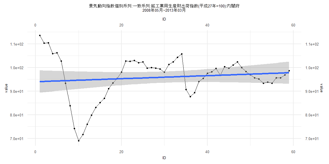
Call:
lm(formula = value ~ ID)

Residuals:
    Min      1Q  Median      3Q     Max
-25.647  -3.846   1.023   5.337  19.532

Coefficients:
            Estimate Std. Error t value            Pr(>|t|)
(Intercept) 94.00362    2.40689  39.056 <0.0000000000000002 ***
ID           0.06434    0.06977   0.922                0.36
---
Signif. codes:  0 '***' 0.001 '**' 0.01 '*' 0.05 '.' 0.1 ' ' 1

Residual standard error: 9.127 on 57 degrees of freedom
Multiple R-squared:  0.0147,    Adjusted R-squared:  -0.002586
F-statistic: 0.8504 on 1 and 57 DF,  p-value: 0.3603


    Two-sample Kolmogorov-Smirnov test

data:  lm_residuals and rnorm(n = length(lm_residuals), mean = 0, sd = sd(lm_residuals))
D = 0.13559, p-value = 0.6544
alternative hypothesis: two-sided


    Durbin-Watson test

data:  value ~ ID
DW = 0.17062, p-value < 0.00000000000000022
alternative hypothesis: true autocorrelation is greater than 0


    studentized Breusch-Pagan test

data:  value ~ ID
BP = 20.77, df = 1, p-value = 0.000005178


    Box-Ljung test

data:  lm_residuals
X-squared = 47.446, df = 1, p-value = 0.000000000005654
Call:
lm(formula = value ~ ID)

Residuals:
    Min      1Q  Median      3Q     Max
-3.7460 -1.3036  0.0081  1.4675  4.1366

Coefficients:
             Estimate Std. Error t value             Pr(>|t|)
(Intercept) 99.879154   0.409566 243.866 < 0.0000000000000002 ***
ID           0.050512   0.009008   5.607          0.000000317 ***
---
Signif. codes:  0 '***' 0.001 '**' 0.01 '*' 0.05 '.' 0.1 ' ' 1

Residual standard error: 1.791 on 76 degrees of freedom
Multiple R-squared:  0.2926,    Adjusted R-squared:  0.2833
F-statistic: 31.44 on 1 and 76 DF,  p-value: 0.0000003167


    Two-sample Kolmogorov-Smirnov test

data:  lm_residuals and rnorm(n = length(lm_residuals), mean = 0, sd = sd(lm_residuals))
D = 0.076923, p-value = 0.9766
alternative hypothesis: two-sided


    Durbin-Watson test

data:  value ~ ID
DW = 0.68868, p-value = 0.000000000006239
alternative hypothesis: true autocorrelation is greater than 0


    studentized Breusch-Pagan test

data:  value ~ ID
BP = 1.1403, df = 1, p-value = 0.2856


    Box-Ljung test

data:  lm_residuals
X-squared = 33.546, df = 1, p-value = 0.00000000696