Analysis
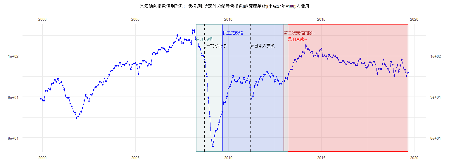
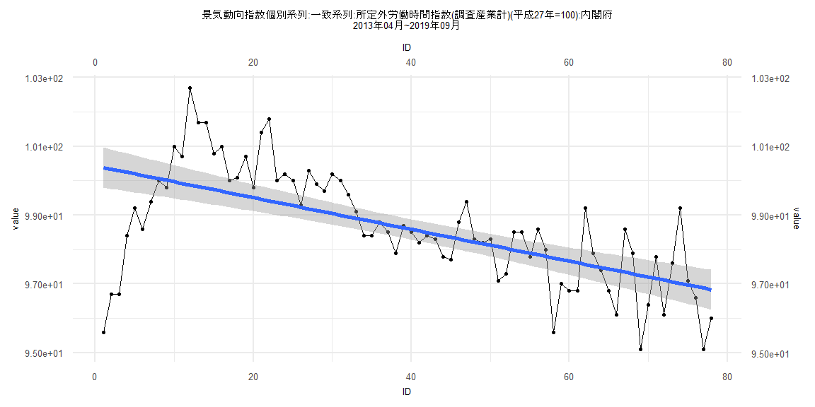
[1] "景気動向指数個別系列:一致系列:所定外労働時間指数(調査産業計)(平成27年=100):内閣府"
       Jan   Feb   Mar   Apr   May   Jun   Jul   Aug   Sep   Oct   Nov   Dec
1999                                                                    89.6
2000  89.3  89.1  91.6  91.5  92.1  91.8  93.1  93.4  94.3  93.7  94.5  93.3
2001  93.6  92.8  91.9  90.3  89.8  89.8  88.4  87.7  86.5  86.2  84.9  85.2
2002  85.8  86.4  87.3  89.1  90.5  89.8  89.0  90.6  90.5  91.7  92.4  92.5
2003  93.0  93.7  93.5  93.0  94.5  93.8  94.5  95.4  96.3  96.5  96.9  97.6
2004  97.6  97.6  98.4  97.5  97.9  97.8  98.2  98.6  97.9  96.7  97.9  98.2
2005  98.3  97.8  95.6  98.2  98.1  98.8  98.9  98.5  97.6  98.2  97.8 100.5
2006 100.8 100.5 100.7 101.5 101.5 102.0 101.9 101.7 101.0 101.0 102.2 102.1
2007 102.6 103.4 103.5 105.1 103.8 104.4 103.2 103.2 104.1 103.9 103.9 103.9
2008 102.9 106.3 106.3 104.1 104.0 102.4 101.7 100.1 100.0  98.5  95.0  89.8
2009  85.2  79.3  78.0  80.5  81.8  82.2  83.9  85.2  86.4  88.7  88.7  90.1
2010  92.1  92.5  93.6  95.3  94.1  93.7  93.9  94.6  93.5  93.3  94.8  93.6
2011  94.0  95.3  92.4  89.6  90.2  92.7  93.8  92.9  94.4  94.9  94.2  95.4
2012  95.5  96.1  95.8  94.9  95.8  95.2  93.7  95.0  94.0  93.2  93.2  93.8
2013  93.9  94.6  94.4  95.6  96.7  96.7  98.4  99.2  98.6  99.4 100.0  99.8
2014 101.0 100.7 102.7 101.7 101.7 100.8 101.0 100.0 100.1 100.7  99.8 101.4
2015 101.8 100.0 100.2 100.0  99.3 100.3  99.9  99.7 100.2 100.0  99.6  99.1
2016  98.4  98.4  98.8  98.5  97.9  98.7  98.5  98.2  98.4  98.3  97.8  97.7
2017  98.8  99.4  98.3  98.2  98.3  97.1  97.3  98.5  98.5  97.8  98.6  98.0
2018  95.6  97.0  96.8  96.8  99.2  97.9  97.4  96.8  96.1  98.6  97.9  95.1
2019  96.4  97.8  96.1  97.6  99.2  97.1  96.6  95.1  96.0
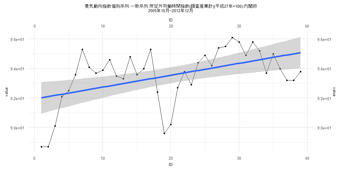
Call:
lm(formula = value ~ ID)

Residuals:
    Min      1Q  Median      3Q     Max
-3.8706 -0.9564  0.4522  1.2294  2.7977

Coefficients:
            Estimate Std. Error t value             Pr(>|t|)
(Intercept) 91.93752    0.54440 168.879 < 0.0000000000000002 ***
ID           0.08069    0.02372   3.401              0.00162 **
---
Signif. codes:  0 '***' 0.001 '**' 0.01 '*' 0.05 '.' 0.1 ' ' 1

Residual standard error: 1.667 on 37 degrees of freedom
Multiple R-squared:  0.2382,    Adjusted R-squared:  0.2176
F-statistic: 11.57 on 1 and 37 DF,  p-value: 0.001622


    Two-sample Kolmogorov-Smirnov test

data:  lm_residuals and rnorm(n = length(lm_residuals), mean = 0, sd = sd(lm_residuals))
D = 0.10256, p-value = 0.9885
alternative hypothesis: two-sided


    Durbin-Watson test

data:  value ~ ID
DW = 0.54693, p-value = 0.000000007334
alternative hypothesis: true autocorrelation is greater than 0


    studentized Breusch-Pagan test

data:  value ~ ID
BP = 3.4199, df = 1, p-value = 0.06442


    Box-Ljung test

data:  lm_residuals
X-squared = 18.608, df = 1, p-value = 0.00001605
Call:
lm(formula = value ~ ID)

Residuals:
    Min      1Q  Median      3Q     Max
-5.7422 -0.7336  0.1920  1.0536  3.4748

Coefficients:
             Estimate Std. Error t value             Pr(>|t|)
(Intercept) 99.672006   0.381066  261.56 < 0.0000000000000002 ***
ID          -0.029790   0.008074   -3.69             0.000411 ***
---
Signif. codes:  0 '***' 0.001 '**' 0.01 '*' 0.05 '.' 0.1 ' ' 1

Residual standard error: 1.699 on 79 degrees of freedom
Multiple R-squared:  0.147, Adjusted R-squared:  0.1362
F-statistic: 13.61 on 1 and 79 DF,  p-value: 0.0004108


    Two-sample Kolmogorov-Smirnov test

data:  lm_residuals and rnorm(n = length(lm_residuals), mean = 0, sd = sd(lm_residuals))
D = 0.22222, p-value = 0.03633
alternative hypothesis: two-sided


    Durbin-Watson test

data:  value ~ ID
DW = 0.3756, p-value < 0.00000000000000022
alternative hypothesis: true autocorrelation is greater than 0


    studentized Breusch-Pagan test

data:  value ~ ID
BP = 16.127, df = 1, p-value = 0.00005924


    Box-Ljung test

data:  lm_residuals
X-squared = 45.575, df = 1, p-value = 0.00000000001469
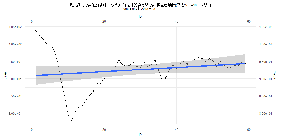
Call:
lm(formula = value ~ ID)

Residuals:
     Min       1Q   Median       3Q      Max
-13.5046  -1.2231   0.6661   1.9542  13.0898

Coefficients:
            Estimate Std. Error t value            Pr(>|t|)
(Intercept) 90.85073    1.38490  65.601 <0.0000000000000002 ***
ID           0.05944    0.04015   1.481               0.144
---
Signif. codes:  0 '***' 0.001 '**' 0.01 '*' 0.05 '.' 0.1 ' ' 1

Residual standard error: 5.251 on 57 degrees of freedom
Multiple R-squared:  0.03703,   Adjusted R-squared:  0.02014
F-statistic: 2.192 on 1 and 57 DF,  p-value: 0.1442


    Two-sample Kolmogorov-Smirnov test

data:  lm_residuals and rnorm(n = length(lm_residuals), mean = 0, sd = sd(lm_residuals))
D = 0.28814, p-value = 0.01452
alternative hypothesis: two-sided


    Durbin-Watson test

data:  value ~ ID
DW = 0.11639, p-value < 0.00000000000000022
alternative hypothesis: true autocorrelation is greater than 0


    studentized Breusch-Pagan test

data:  value ~ ID
BP = 26.438, df = 1, p-value = 0.0000002721


    Box-Ljung test

data:  lm_residuals
X-squared = 48.854, df = 1, p-value = 0.000000000002758
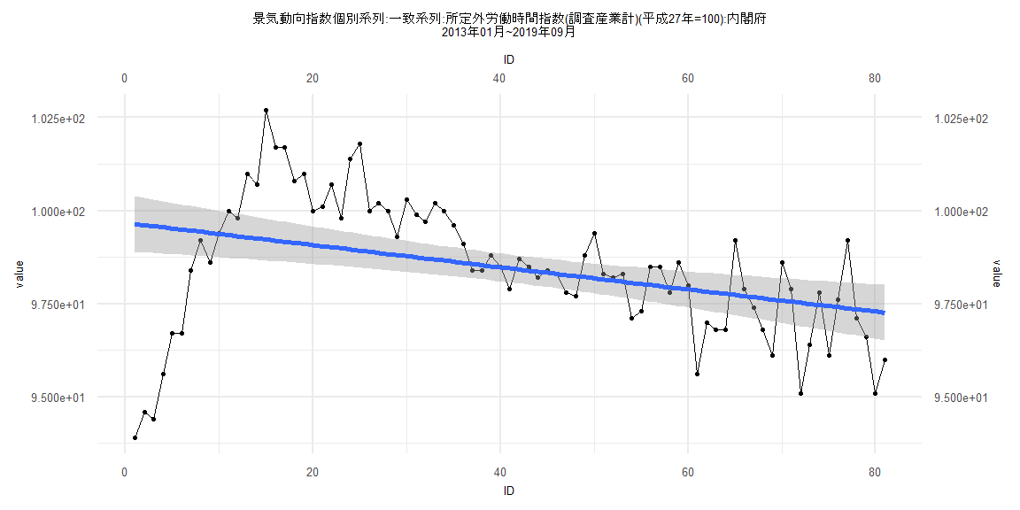
Call:
lm(formula = value ~ ID)

Residuals:
    Min      1Q  Median      3Q     Max
-4.7862 -0.6962  0.0744  0.7434  2.8212

Coefficients:
              Estimate Std. Error t value             Pr(>|t|)
(Intercept) 100.432334   0.298191 336.806 < 0.0000000000000002 ***
ID           -0.046129   0.006559  -7.033        0.00000000076 ***
---
Signif. codes:  0 '***' 0.001 '**' 0.01 '*' 0.05 '.' 0.1 ' ' 1

Residual standard error: 1.304 on 76 degrees of freedom
Multiple R-squared:  0.3943,    Adjusted R-squared:  0.3863
F-statistic: 49.47 on 1 and 76 DF,  p-value: 0.0000000007597


    Two-sample Kolmogorov-Smirnov test

data:  lm_residuals and rnorm(n = length(lm_residuals), mean = 0, sd = sd(lm_residuals))
D = 0.11538, p-value = 0.6802
alternative hypothesis: two-sided


    Durbin-Watson test

data:  value ~ ID
DW = 0.64739, p-value = 0.0000000000008209
alternative hypothesis: true autocorrelation is greater than 0


    studentized Breusch-Pagan test

data:  value ~ ID
BP = 8.9208, df = 1, p-value = 0.002819


    Box-Ljung test

data:  lm_residuals
X-squared = 27.733, df = 1, p-value = 0.0000001392