Analysis
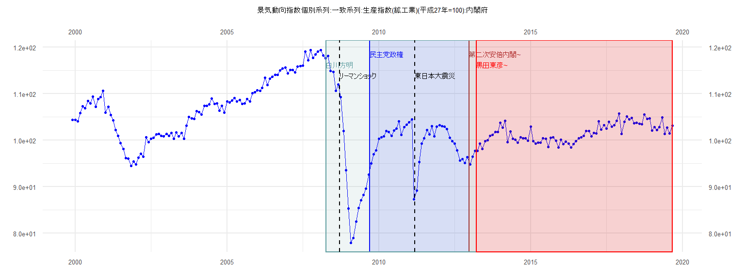
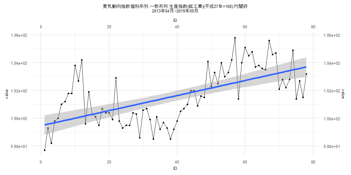
[1] "景気動向指数個別系列:一致系列:生産指数(鉱工業)(平成27年=100):内閣府"
       Jan   Feb   Mar   Apr   May   Jun   Jul   Aug   Sep   Oct   Nov   Dec
1999                                                                   104.4
2000 104.4 104.1 105.9 107.3 106.9 108.5 107.9 109.4 107.2 108.9 109.3 110.7
2001 106.0 107.2 105.4 104.3 102.2 101.0  99.4  98.2  96.2  96.1  94.5  95.5
2002  94.8  96.3  97.1  96.5 100.7  99.6 100.3 100.6 101.3 101.4 101.0 100.9
2003 101.4 101.0 101.6 100.3 101.7 100.9 101.6 100.3 103.2 105.0 104.7 104.6
2004 106.3 106.1 105.6 107.4 107.4 107.7 109.0 107.8 108.0 106.4 107.4 106.0
2005 108.4 108.2 108.6 109.1 108.4 108.7 107.8 107.9 108.9 108.4 110.1 110.3
2006 110.8 110.7 111.3 113.5 111.9 113.3 113.7 114.1 114.1 115.0 115.4 115.7
2007 114.4 115.1 115.1 114.6 115.9 116.0 116.1 119.1 117.2 119.4 117.7 118.5
2008 119.1 119.4 118.3 117.6 118.2 114.9 114.7 110.7 112.0 109.3 102.0  93.6
2009  85.3  78.0  79.0  82.5  85.5  87.1  88.3  89.6  92.6  95.0  97.0  97.8
2010 100.3 100.7 100.9 102.0 101.8 101.0 102.1 102.5 104.1 101.2 102.8 103.4
2011 103.9 104.5  87.3  89.2  95.3  99.3 100.5 102.2 101.3 103.1 100.9 102.9
2012 103.3 103.1 102.9 102.4 100.6  99.8  99.3  97.8  95.7  96.0  95.1  96.4
2013  94.8  96.5  97.7  97.7  99.3  98.2  99.8 100.0 101.0 101.2 101.8 101.8
2014 103.8 102.7 104.2  99.6 101.9 100.3 100.1  99.5 100.7 100.4 100.4  99.9
2015 102.9  99.8  99.3  99.5  99.5 100.4 100.3  98.6 100.6 100.7  99.9  98.5
2016 100.1  99.2  99.7  99.3  98.5  99.2  99.8 100.5 100.7 101.0 102.0 102.0
2017 100.9 101.6 101.5 104.1 102.3 103.3 102.5 104.0 103.0 103.3 104.2 105.8
2018 101.4 104.0 105.1 104.5 104.8 103.7 103.8 103.6 103.5 105.6 104.6 104.7
2019 102.1 102.8 102.2 102.8 104.9 101.4 102.7 101.5 103.2
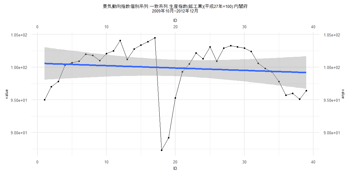
Call:
lm(formula = value ~ ID)

Residuals:
    Min      1Q  Median      3Q     Max
-12.655  -2.119   1.063   2.809   4.509

Coefficients:
             Estimate Std. Error t value            Pr(>|t|)
(Intercept) 100.61120    1.27380  78.985 <0.0000000000000002 ***
ID           -0.03646    0.05551  -0.657               0.515
---
Signif. codes:  0 '***' 0.001 '**' 0.01 '*' 0.05 '.' 0.1 ' ' 1

Residual standard error: 3.901 on 37 degrees of freedom
Multiple R-squared:  0.01153,   Adjusted R-squared:  -0.01519
F-statistic: 0.4314 on 1 and 37 DF,  p-value: 0.5154


    Two-sample Kolmogorov-Smirnov test

data:  lm_residuals and rnorm(n = length(lm_residuals), mean = 0, sd = sd(lm_residuals))
D = 0.17949, p-value = 0.5622
alternative hypothesis: two-sided


    Durbin-Watson test

data:  value ~ ID
DW = 0.73299, p-value = 0.000001258
alternative hypothesis: true autocorrelation is greater than 0


    studentized Breusch-Pagan test

data:  value ~ ID
BP = 0.033081, df = 1, p-value = 0.8557


    Box-Ljung test

data:  lm_residuals
X-squared = 15.098, df = 1, p-value = 0.0001021
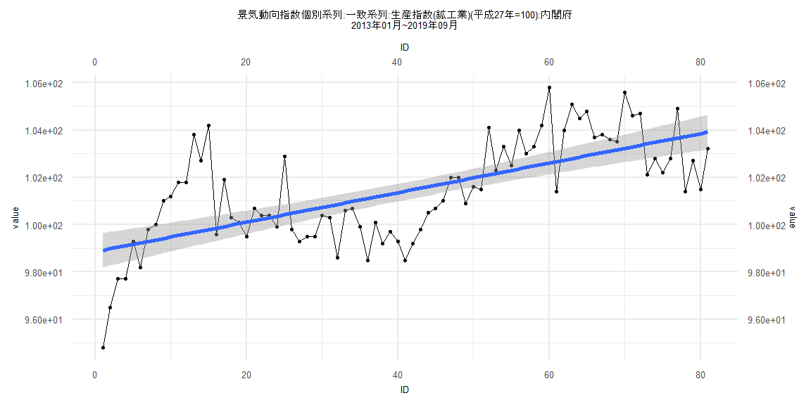
Call:
lm(formula = value ~ ID)

Residuals:
    Min      1Q  Median      3Q     Max
-4.1147 -1.1037 -0.2527  1.2327  4.4098

Coefficients:
             Estimate Std. Error t value             Pr(>|t|)
(Intercept) 98.852160   0.372485 265.385 < 0.0000000000000002 ***
ID           0.062534   0.007892   7.924      0.0000000000123 ***
---
Signif. codes:  0 '***' 0.001 '**' 0.01 '*' 0.05 '.' 0.1 ' ' 1

Residual standard error: 1.661 on 79 degrees of freedom
Multiple R-squared:  0.4428,    Adjusted R-squared:  0.4358
F-statistic: 62.79 on 1 and 79 DF,  p-value: 0.00000000001227


    Two-sample Kolmogorov-Smirnov test

data:  lm_residuals and rnorm(n = length(lm_residuals), mean = 0, sd = sd(lm_residuals))
D = 0.19753, p-value = 0.08471
alternative hypothesis: two-sided


    Durbin-Watson test

data:  value ~ ID
DW = 0.78625, p-value = 0.0000000002108
alternative hypothesis: true autocorrelation is greater than 0


    studentized Breusch-Pagan test

data:  value ~ ID
BP = 3.4648, df = 1, p-value = 0.06269


    Box-Ljung test

data:  lm_residuals
X-squared = 27.002, df = 1, p-value = 0.0000002033
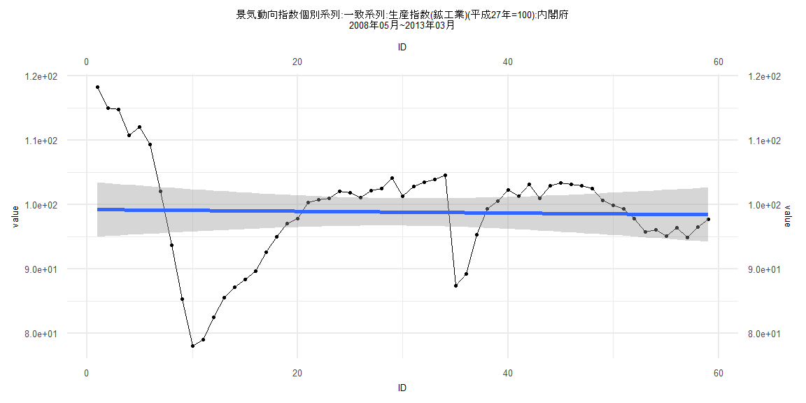
Call:
lm(formula = value ~ ID)

Residuals:
    Min      1Q  Median      3Q     Max
-21.047  -3.357   1.848   4.178  19.030

Coefficients:
            Estimate Std. Error t value            Pr(>|t|)
(Intercept) 99.18311    2.15502  46.024 <0.0000000000000002 ***
ID          -0.01362    0.06247  -0.218               0.828
---
Signif. codes:  0 '***' 0.001 '**' 0.01 '*' 0.05 '.' 0.1 ' ' 1

Residual standard error: 8.172 on 57 degrees of freedom
Multiple R-squared:  0.0008329, Adjusted R-squared:  -0.0167
F-statistic: 0.04752 on 1 and 57 DF,  p-value: 0.8282


    Two-sample Kolmogorov-Smirnov test

data:  lm_residuals and rnorm(n = length(lm_residuals), mean = 0, sd = sd(lm_residuals))
D = 0.23729, p-value = 0.07193
alternative hypothesis: two-sided


    Durbin-Watson test

data:  value ~ ID
DW = 0.19537, p-value < 0.00000000000000022
alternative hypothesis: true autocorrelation is greater than 0


    studentized Breusch-Pagan test

data:  value ~ ID
BP = 22.651, df = 1, p-value = 0.000001943


    Box-Ljung test

data:  lm_residuals
X-squared = 45.327, df = 1, p-value = 0.00000000001667
Call:
lm(formula = value ~ ID)

Residuals:
    Min      1Q  Median      3Q     Max
-3.0300 -1.1754 -0.2542  1.2988  4.0828

Coefficients:
             Estimate Std. Error t value             Pr(>|t|)
(Intercept) 99.465135   0.361099 275.451 < 0.0000000000000002 ***
ID           0.054339   0.007942   6.842        0.00000000174 ***
---
Signif. codes:  0 '***' 0.001 '**' 0.01 '*' 0.05 '.' 0.1 ' ' 1

Residual standard error: 1.579 on 76 degrees of freedom
Multiple R-squared:  0.3812,    Adjusted R-squared:  0.373
F-statistic: 46.81 on 1 and 76 DF,  p-value: 0.000000001741


    Two-sample Kolmogorov-Smirnov test

data:  lm_residuals and rnorm(n = length(lm_residuals), mean = 0, sd = sd(lm_residuals))
D = 0.15385, p-value = 0.316
alternative hypothesis: two-sided


    Durbin-Watson test

data:  value ~ ID
DW = 0.88283, p-value = 0.00000001459
alternative hypothesis: true autocorrelation is greater than 0


    studentized Breusch-Pagan test

data:  value ~ ID
BP = 0.75896, df = 1, p-value = 0.3837


    Box-Ljung test

data:  lm_residuals
X-squared = 24.441, df = 1, p-value = 0.000000766