Analysis
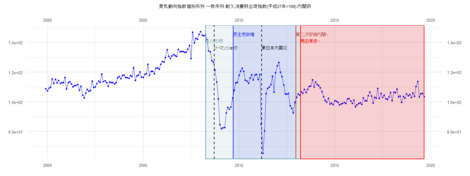
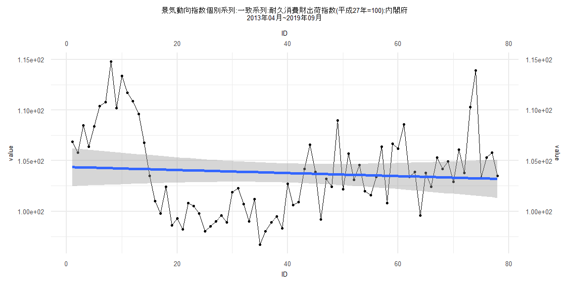
[1] "景気動向指数個別系列:一致系列:耐久消費財出荷指数(平成27年=100):内閣府"
       Jan   Feb   Mar   Apr   May   Jun   Jul   Aug   Sep   Oct   Nov   Dec
1999                                                                   108.8
2000 107.4 109.3 109.9 115.4 112.4 115.2 112.8 114.5 112.4 113.1 113.0 116.6
2001 108.7 113.1 113.7 112.1 110.2 111.0 111.1 111.7 107.8 110.5 104.6 102.7
2002 105.9 108.5 107.3 107.7 114.0 109.8 110.2 112.4 114.1 113.3 118.7 113.7
2003 114.2 113.0 110.5 113.4 113.0 113.1 112.2 113.0 116.4 117.2 115.7 117.7
2004 118.2 116.5 116.4 115.9 117.7 117.2 123.2 114.4 117.5 118.2 120.2 116.7
2005 116.5 118.6 118.9 125.4 118.0 120.7 120.7 118.9 122.7 122.8 122.0 125.4
2006 127.3 126.8 129.9 135.2 130.8 129.2 130.9 132.0 131.2 130.8 135.4 133.8
2007 134.0 134.1 133.4 133.6 135.4 138.2 129.3 147.0 139.8 142.8 142.3 145.5
2008 147.4 145.0 144.5 145.2 142.1 134.5 133.8 127.9 126.8 121.4 113.4 102.1
2009  84.7  81.8  82.5  82.7  92.6  96.4  95.0  96.6 102.6 107.9 112.7 113.3
2010 118.0 120.8 122.6 120.6 114.7 114.1 112.5 116.1 118.4 114.8 118.2 118.5
2011 115.0 118.6  84.9  65.5  80.4 105.5 109.1 110.2 111.8 117.4 106.6 119.9
2012 124.4 126.6 120.0 117.1 111.4 105.3 105.1 105.7  97.3  95.7  92.6  99.6
2013 103.1 105.3 104.6 106.9 105.8 108.5 106.4 108.4 110.4 110.8 114.8 110.2
2014 113.4 111.7 110.9 109.6 106.8 103.5 101.0  99.8 102.4  98.6  99.3  98.2
2015 100.8 100.5  99.8  98.0  98.5  99.0  99.6  98.9 101.9 102.3 100.7  99.0
2016 101.2  96.7  98.0  98.9  99.5  98.3 102.7 100.6 100.9 104.2 106.6 103.9
2017  99.2 103.2 102.4 109.0 102.2 105.7 103.1 104.6 102.0 101.6 103.4 106.4
2018 100.8 106.7 106.2 108.6 103.4 103.9  99.6 103.8 102.4 105.3 104.2 104.9
2019 102.9 106.1 103.8 110.3 113.9 103.3 105.3 105.8 103.5
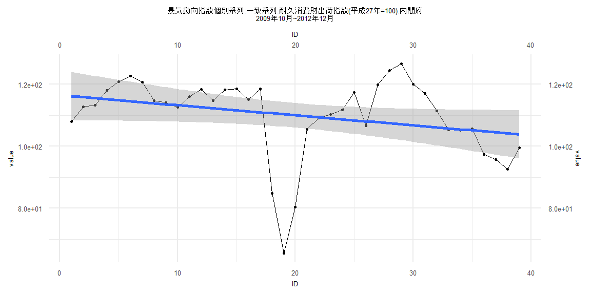
Call:
lm(formula = value ~ ID)

Residuals:
    Min      1Q  Median      3Q     Max
-44.795  -2.634   1.199   6.354  19.540

Coefficients:
            Estimate Std. Error t value            Pr(>|t|)
(Intercept) 116.4430     3.9893  29.189 <0.0000000000000002 ***
ID           -0.3236     0.1738  -1.861              0.0707 .
---
Signif. codes:  0 '***' 0.001 '**' 0.01 '*' 0.05 '.' 0.1 ' ' 1

Residual standard error: 12.22 on 37 degrees of freedom
Multiple R-squared:  0.08562,   Adjusted R-squared:  0.06091
F-statistic: 3.465 on 1 and 37 DF,  p-value: 0.07065


    Two-sample Kolmogorov-Smirnov test

data:  lm_residuals and rnorm(n = length(lm_residuals), mean = 0, sd = sd(lm_residuals))
D = 0.28205, p-value = 0.08974
alternative hypothesis: two-sided


    Durbin-Watson test

data:  value ~ ID
DW = 0.57024, p-value = 0.0000000156
alternative hypothesis: true autocorrelation is greater than 0


    studentized Breusch-Pagan test

data:  value ~ ID
BP = 0.091639, df = 1, p-value = 0.7621


    Box-Ljung test

data:  lm_residuals
X-squared = 21.042, df = 1, p-value = 0.000004493
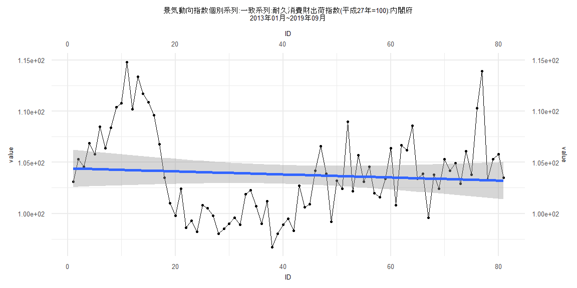
Call:
lm(formula = value ~ ID)

Residuals:
   Min     1Q Median     3Q    Max
-7.152 -3.197 -0.139  2.574 10.629

Coefficients:
             Estimate Std. Error t value            Pr(>|t|)
(Intercept) 104.41870    0.92907 112.390 <0.0000000000000002 ***
ID           -0.01491    0.01968  -0.757               0.451
---
Signif. codes:  0 '***' 0.001 '**' 0.01 '*' 0.05 '.' 0.1 ' ' 1

Residual standard error: 4.142 on 79 degrees of freedom
Multiple R-squared:  0.00721,   Adjusted R-squared:  -0.005357
F-statistic: 0.5737 on 1 and 79 DF,  p-value: 0.451


    Two-sample Kolmogorov-Smirnov test

data:  lm_residuals and rnorm(n = length(lm_residuals), mean = 0, sd = sd(lm_residuals))
D = 0.098765, p-value = 0.8277
alternative hypothesis: two-sided


    Durbin-Watson test

data:  value ~ ID
DW = 0.5538, p-value = 0.000000000000001387
alternative hypothesis: true autocorrelation is greater than 0


    studentized Breusch-Pagan test

data:  value ~ ID
BP = 4.7687, df = 1, p-value = 0.02898


    Box-Ljung test

data:  lm_residuals
X-squared = 43.861, df = 1, p-value = 0.00000000003525
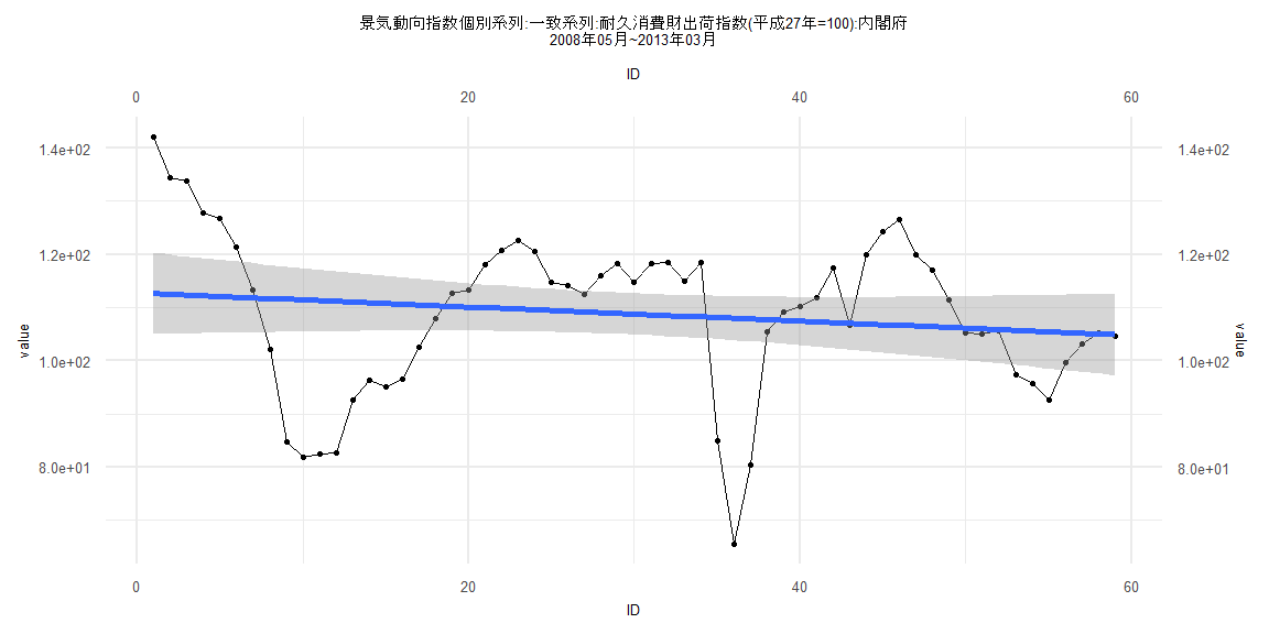
Call:
lm(formula = value ~ ID)

Residuals:
    Min      1Q  Median      3Q     Max
-42.496  -8.179   2.735  10.086  29.456

Coefficients:
            Estimate Std. Error t value            Pr(>|t|)
(Intercept) 112.7770     3.9271  28.718 <0.0000000000000002 ***
ID           -0.1328     0.1138  -1.166               0.248
---
Signif. codes:  0 '***' 0.001 '**' 0.01 '*' 0.05 '.' 0.1 ' ' 1

Residual standard error: 14.89 on 57 degrees of freedom
Multiple R-squared:  0.02332,   Adjusted R-squared:  0.00618
F-statistic: 1.361 on 1 and 57 DF,  p-value: 0.2483


    Two-sample Kolmogorov-Smirnov test

data:  lm_residuals and rnorm(n = length(lm_residuals), mean = 0, sd = sd(lm_residuals))
D = 0.28814, p-value = 0.01452
alternative hypothesis: two-sided


    Durbin-Watson test

data:  value ~ ID
DW = 0.3139, p-value < 0.00000000000000022
alternative hypothesis: true autocorrelation is greater than 0


    studentized Breusch-Pagan test

data:  value ~ ID
BP = 5.7816, df = 1, p-value = 0.01619


    Box-Ljung test

data:  lm_residuals
X-squared = 40.584, df = 1, p-value = 0.0000000001884
Call:
lm(formula = value ~ ID)

Residuals:
    Min      1Q  Median      3Q     Max
-7.1552 -3.2390 -0.2819  2.6154 10.6344

Coefficients:
             Estimate Std. Error t value            Pr(>|t|)
(Intercept) 104.38438    0.96470 108.204 <0.0000000000000002 ***
ID           -0.01512    0.02122  -0.713               0.478
---
Signif. codes:  0 '***' 0.001 '**' 0.01 '*' 0.05 '.' 0.1 ' ' 1

Residual standard error: 4.219 on 76 degrees of freedom
Multiple R-squared:  0.006636,  Adjusted R-squared:  -0.006434
F-statistic: 0.5077 on 1 and 76 DF,  p-value: 0.4783


    Two-sample Kolmogorov-Smirnov test

data:  lm_residuals and rnorm(n = length(lm_residuals), mean = 0, sd = sd(lm_residuals))
D = 0.10256, p-value = 0.81
alternative hypothesis: two-sided


    Durbin-Watson test

data:  value ~ ID
DW = 0.54692, p-value = 0.000000000000002773
alternative hypothesis: true autocorrelation is greater than 0


    studentized Breusch-Pagan test

data:  value ~ ID
BP = 7.3808, df = 1, p-value = 0.006592


    Box-Ljung test

data:  lm_residuals
X-squared = 42.495, df = 1, p-value = 0.00000000007086