Analysis
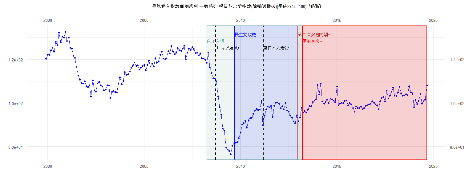
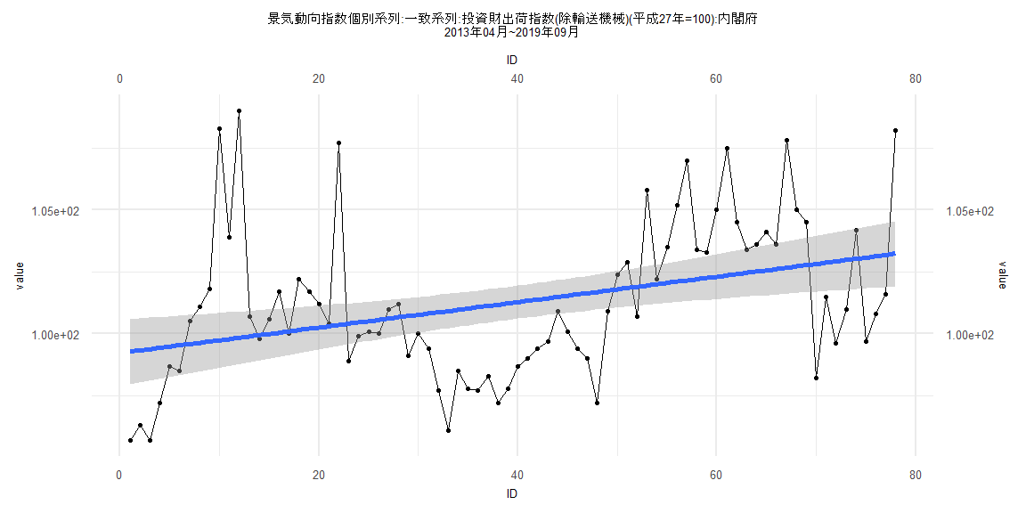
[1] "景気動向指数個別系列:一致系列:投資財出荷指数(除輸送機械)(平成27年=100):内閣府"
       Jan   Feb   Mar   Apr   May   Jun   Jul   Aug   Sep   Oct   Nov   Dec
1999                                                                   120.3
2000 122.1 122.1 124.3 125.4 123.5 128.1 126.6 132.3 127.9 130.4 130.0 132.7
2001 128.5 130.1 125.4 125.0 121.7 120.7 116.4 112.7 110.8 109.2 109.0 110.0
2002 107.8 107.3 108.2 103.0 110.5 105.8 105.3 109.0 109.8 108.0 107.6 105.8
2003 106.2 108.2 108.1 102.1 105.1 105.7 105.1 105.0 108.9 111.8 108.6 110.1
2004 114.2 113.0 113.1 114.6 116.2 117.1 118.6 117.1 117.4 115.4 116.2 117.1
2005 117.5 114.9 117.5 119.5 116.8 118.0 116.9 120.6 118.5 119.2 122.1 123.5
2006 120.5 120.1 120.5 123.9 122.9 126.2 123.7 122.4 123.1 125.2 124.3 124.0
2007 124.9 126.3 120.1 123.1 124.9 124.4 125.6 124.8 122.9 123.1 121.9 122.9
2008 120.6 120.5 119.9 118.5 123.3 116.5 113.9 111.5 111.3 110.0 103.1  98.2
2009  94.6  88.3  87.3  79.6  78.7  78.0  76.7  80.4  81.7  81.8  82.2  84.0
2010  86.6  90.2  90.8  91.8  88.8  92.2  93.1  93.2  95.1  96.7  97.3  96.8
2011  97.0 101.0  89.9  94.4  97.0  98.5  98.0  98.7  93.7  98.8 100.1 100.3
2012  99.8  97.6  98.6  97.2 100.0  96.7  96.1  94.2  93.4  91.6  90.7  94.4
2013  91.7  93.4  97.9  95.7  96.3  95.7  97.2  98.7  98.5 100.5 101.1 101.8
2014 108.3 103.9 109.0 100.7  99.8 100.6 101.7 100.0 102.2 101.7 101.2 100.4
2015 107.7  98.9  99.9 100.1 100.0 101.0 101.2  99.1 100.0  99.4  97.7  96.1
2016  98.5  97.8  97.7  98.3  97.2  97.8  98.7  99.0  99.4  99.7 100.9 100.1
2017  99.4  99.0  97.2 100.9 102.4 102.9 100.7 105.8 102.2 103.5 105.2 107.0
2018 103.4 103.3 105.0 107.5 104.5 103.4 103.6 104.1 103.6 107.8 105.0 104.5
2019  98.2 101.5  99.6 101.0 104.2  99.7 100.8 101.6 108.2
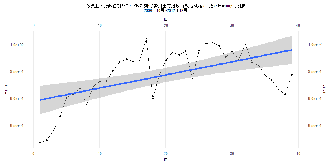
Call:
lm(formula = value ~ ID)

Residuals:
   Min     1Q Median     3Q    Max
-7.995 -3.180  0.648  3.403  7.415

Coefficients:
            Estimate Std. Error t value             Pr(>|t|)
(Intercept) 89.44858    1.33678  66.914 < 0.0000000000000002 ***
ID           0.24334    0.05825   4.178             0.000172 ***
---
Signif. codes:  0 '***' 0.001 '**' 0.01 '*' 0.05 '.' 0.1 ' ' 1

Residual standard error: 4.094 on 37 degrees of freedom
Multiple R-squared:  0.3205,    Adjusted R-squared:  0.3021
F-statistic: 17.45 on 1 and 37 DF,  p-value: 0.0001723


    Two-sample Kolmogorov-Smirnov test

data:  lm_residuals and rnorm(n = length(lm_residuals), mean = 0, sd = sd(lm_residuals))
D = 0.15385, p-value = 0.7523
alternative hypothesis: two-sided


    Durbin-Watson test

data:  value ~ ID
DW = 0.51579, p-value = 0.000000002515
alternative hypothesis: true autocorrelation is greater than 0


    studentized Breusch-Pagan test

data:  value ~ ID
BP = 0.051917, df = 1, p-value = 0.8198


    Box-Ljung test

data:  lm_residuals
X-squared = 19.188, df = 1, p-value = 0.00001184
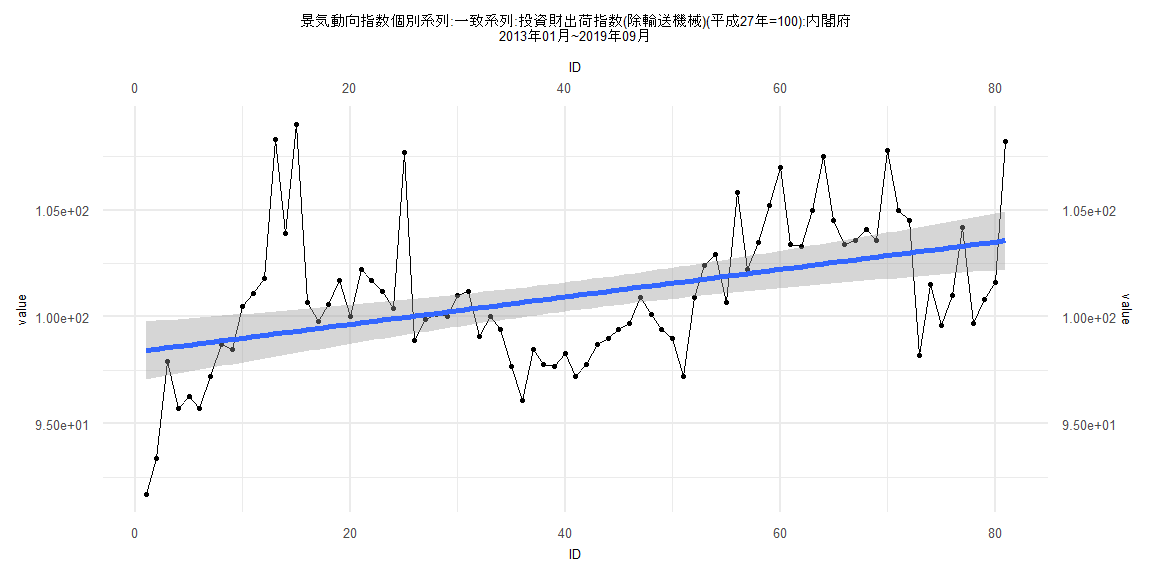
Call:
lm(formula = value ~ ID)

Residuals:
    Min      1Q  Median      3Q     Max
-6.7270 -2.2416 -0.1771  1.4083  9.6729

Coefficients:
            Estimate Std. Error t value             Pr(>|t|)
(Intercept) 98.36275    0.68903 142.756 < 0.0000000000000002 ***
ID           0.06429    0.01460   4.404             0.000033 ***
---
Signif. codes:  0 '***' 0.001 '**' 0.01 '*' 0.05 '.' 0.1 ' ' 1

Residual standard error: 3.072 on 79 degrees of freedom
Multiple R-squared:  0.1971,    Adjusted R-squared:  0.187
F-statistic:  19.4 on 1 and 79 DF,  p-value: 0.00003299


    Two-sample Kolmogorov-Smirnov test

data:  lm_residuals and rnorm(n = length(lm_residuals), mean = 0, sd = sd(lm_residuals))
D = 0.12346, p-value = 0.5705
alternative hypothesis: two-sided


    Durbin-Watson test

data:  value ~ ID
DW = 0.83427, p-value = 0.000000001402
alternative hypothesis: true autocorrelation is greater than 0


    studentized Breusch-Pagan test

data:  value ~ ID
BP = 1.9673, df = 1, p-value = 0.1607


    Box-Ljung test

data:  lm_residuals
X-squared = 24.337, df = 1, p-value = 0.0000008087
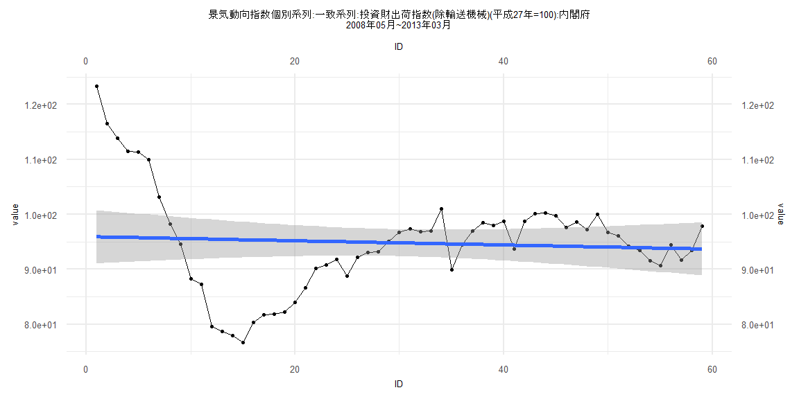
Call:
lm(formula = value ~ ID)

Residuals:
     Min       1Q   Median       3Q      Max
-18.6937  -4.5086   0.2414   4.2250  27.3712

Coefficients:
            Estimate Std. Error t value            Pr(>|t|)
(Intercept) 95.96704    2.47153  38.829 <0.0000000000000002 ***
ID          -0.03822    0.07165  -0.534               0.596
---
Signif. codes:  0 '***' 0.001 '**' 0.01 '*' 0.05 '.' 0.1 ' ' 1

Residual standard error: 9.372 on 57 degrees of freedom
Multiple R-squared:  0.004969,  Adjusted R-squared:  -0.01249
F-statistic: 0.2846 on 1 and 57 DF,  p-value: 0.5958


    Two-sample Kolmogorov-Smirnov test

data:  lm_residuals and rnorm(n = length(lm_residuals), mean = 0, sd = sd(lm_residuals))
D = 0.15254, p-value = 0.5021
alternative hypothesis: two-sided


    Durbin-Watson test

data:  value ~ ID
DW = 0.123, p-value < 0.00000000000000022
alternative hypothesis: true autocorrelation is greater than 0


    studentized Breusch-Pagan test

data:  value ~ ID
BP = 24.742, df = 1, p-value = 0.0000006553


    Box-Ljung test

data:  lm_residuals
X-squared = 46.099, df = 1, p-value = 0.00000000001124
Call:
lm(formula = value ~ ID)

Residuals:
    Min      1Q  Median      3Q     Max
-4.8213 -2.2211 -0.2779  1.4593  9.1573

Coefficients:
            Estimate Std. Error t value             Pr(>|t|)
(Intercept) 99.22631    0.67651 146.673 < 0.0000000000000002 ***
ID           0.05136    0.01488   3.452             0.000912 ***
---
Signif. codes:  0 '***' 0.001 '**' 0.01 '*' 0.05 '.' 0.1 ' ' 1

Residual standard error: 2.959 on 76 degrees of freedom
Multiple R-squared:  0.1355,    Adjusted R-squared:  0.1242
F-statistic: 11.92 on 1 and 76 DF,  p-value: 0.0009124


    Two-sample Kolmogorov-Smirnov test

data:  lm_residuals and rnorm(n = length(lm_residuals), mean = 0, sd = sd(lm_residuals))
D = 0.076923, p-value = 0.9766
alternative hypothesis: two-sided


    Durbin-Watson test

data:  value ~ ID
DW = 0.89386, p-value = 0.00000002109
alternative hypothesis: true autocorrelation is greater than 0


    studentized Breusch-Pagan test

data:  value ~ ID
BP = 0.7244, df = 1, p-value = 0.3947


    Box-Ljung test

data:  lm_residuals
X-squared = 22.328, df = 1, p-value = 0.000002298